Dense Tiling Meets Structured Sparsity
Scalable Algorithms for High-Performance Computing
Esmail Abdul Fattah
esmail.abdulfattah@kaust.edu.sa
King Abdullah University of Science and Technology (KAUST)
Hatem Ltaief, Håvard Rue, David E. Keyes
SIAM Conference on Parallel Processing for Scientific Computing (PP26)
INLA enables fast Bayesian inference for latent Gaussian models, powering research in epidemiology, ecology, climate science, public health, and beyond.
Source: r-inla.org
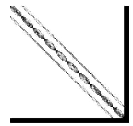
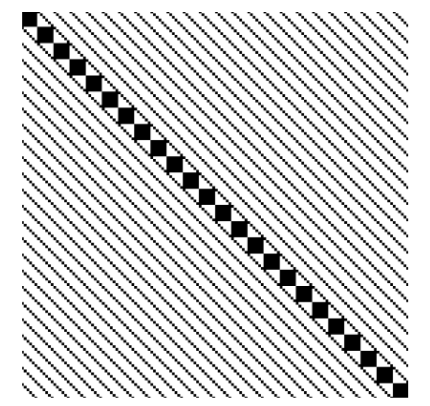
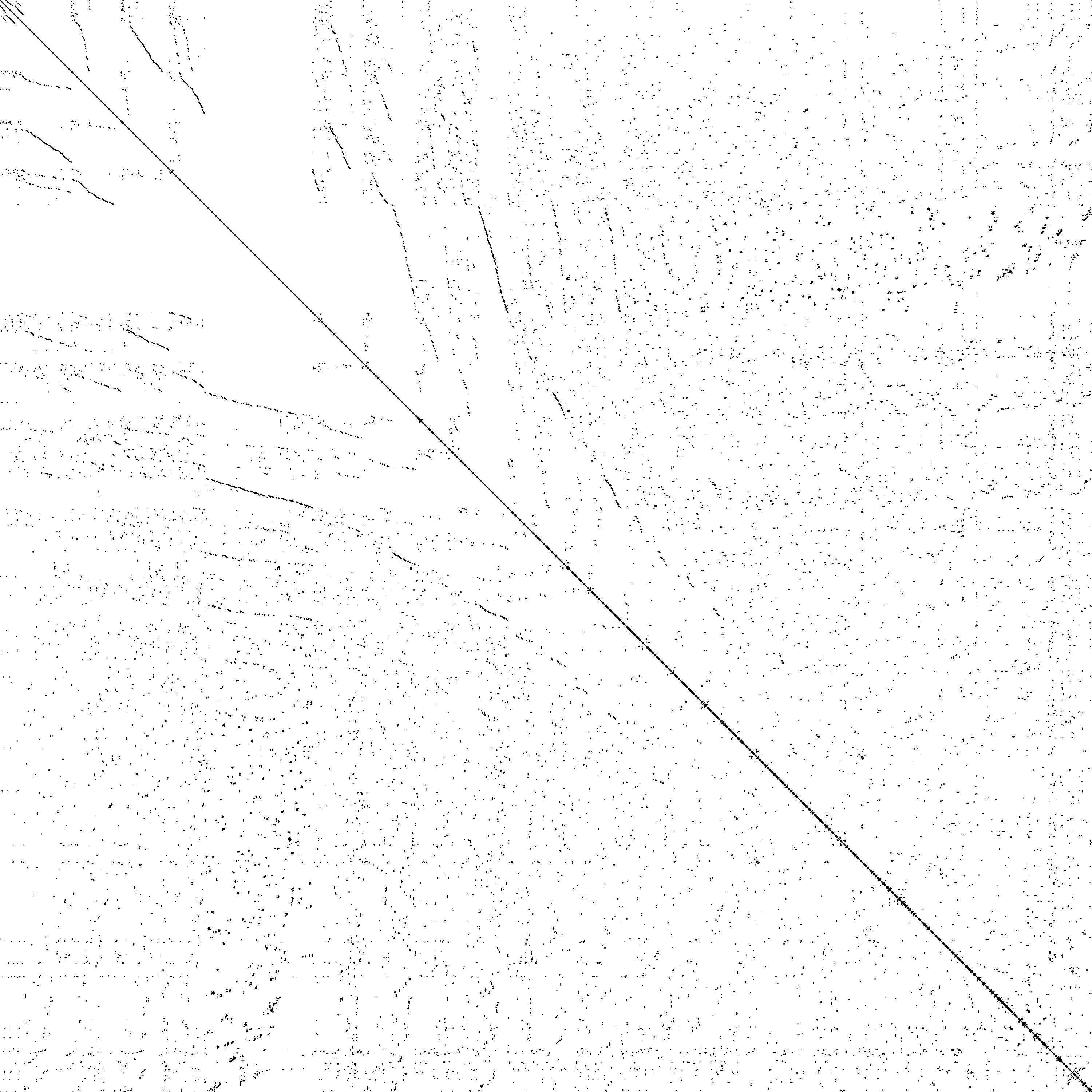
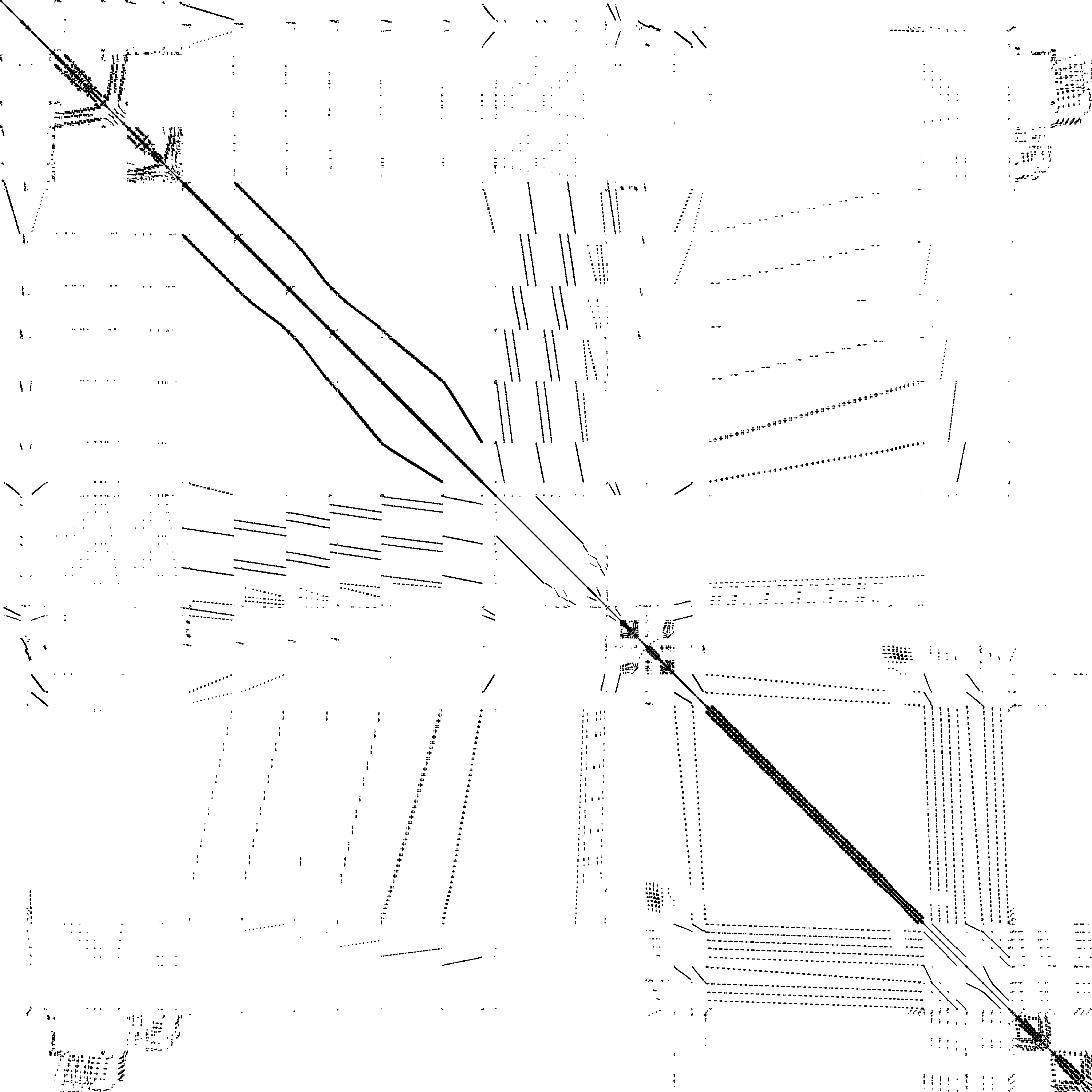
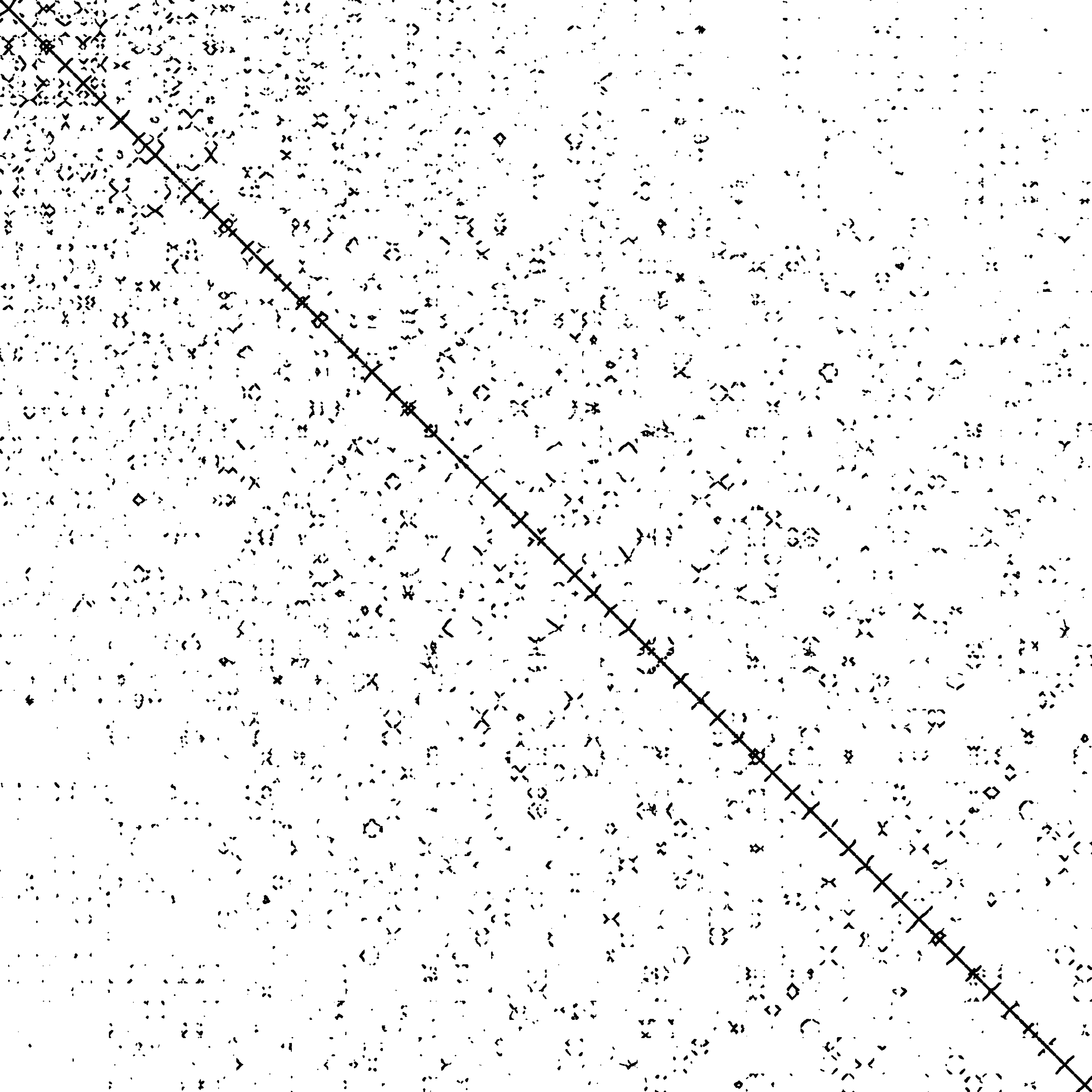
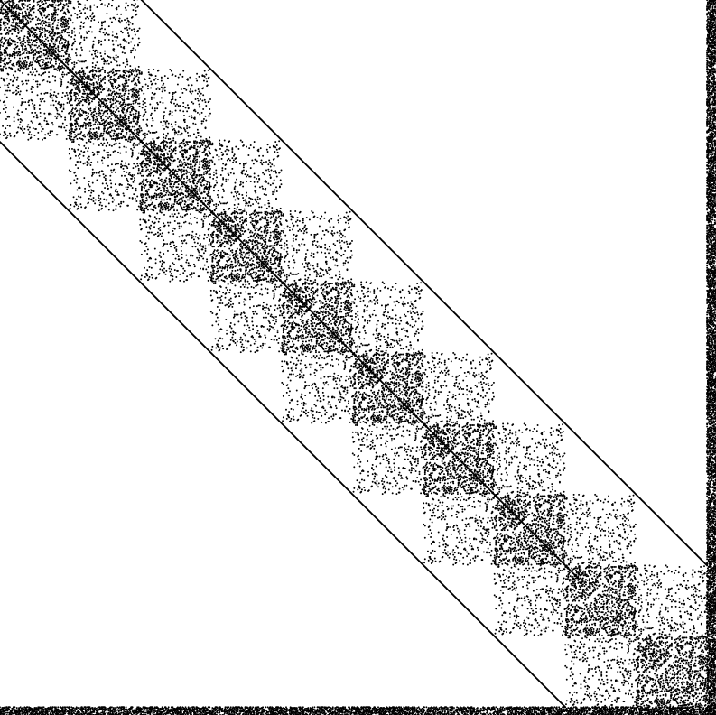
INLA generates diverse structured sparse matrices from Kronecker products of spatial, temporal, and other model components.

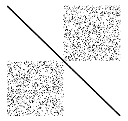
Sparse Solvers
- Low arithmetic intensity
- Poor cache utilization
- Irregular memory access
Dense Solvers
- O(n³) complexity
- Ignores sparsity pattern
- Wastes memory on zeros
Neither approach is optimal! We need the efficiency of sparse + the performance of dense.
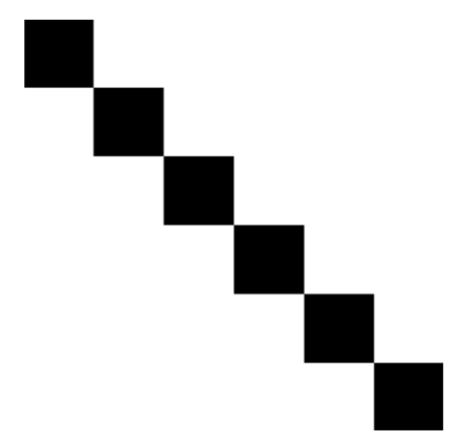
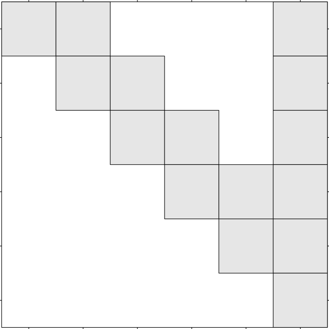
sTiles = Hybrid framework combining sparse techniques (ordering, skip zeros) with dense performance (LAPACK/BLAS-3 on tiles)
Sparse Points
Dense Tiles
LAPACK/BLAS-3
Skip zero tiles
44 / 100
tiles computed
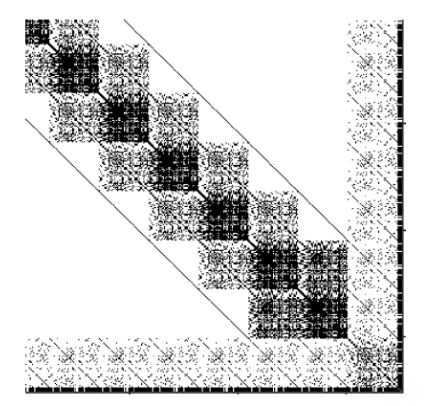
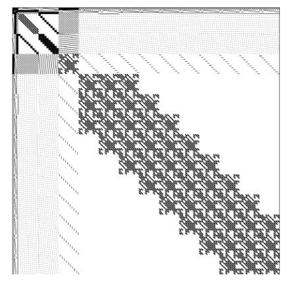
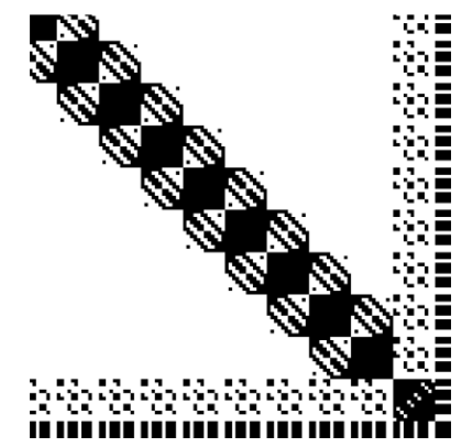
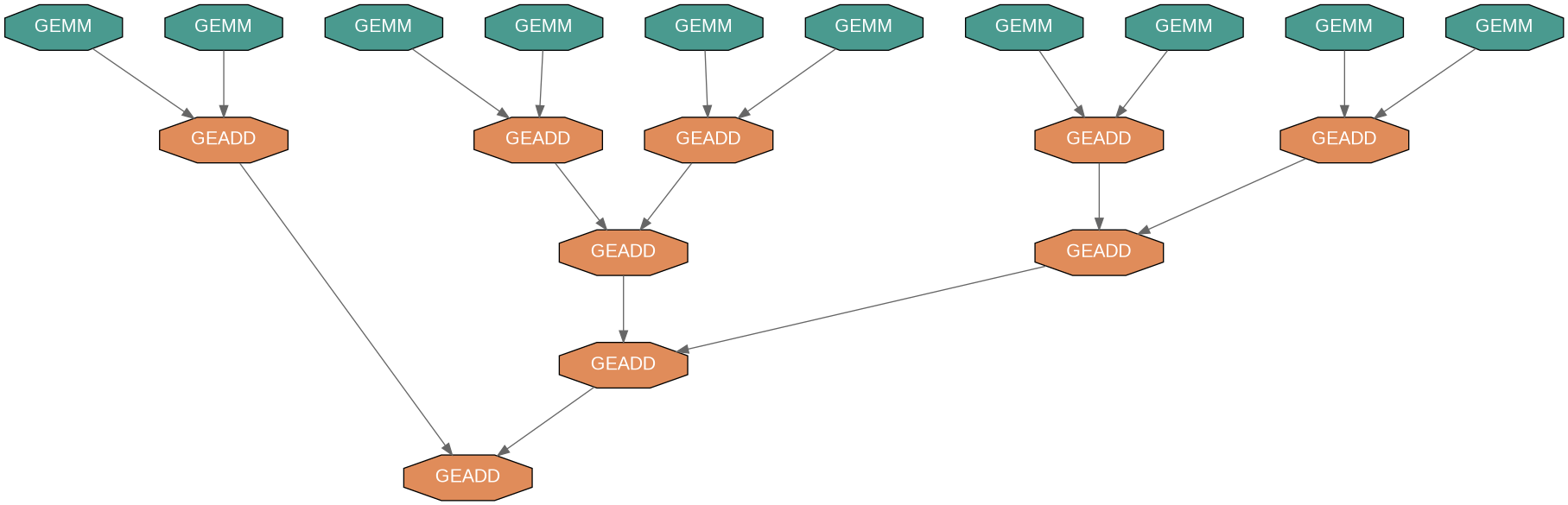
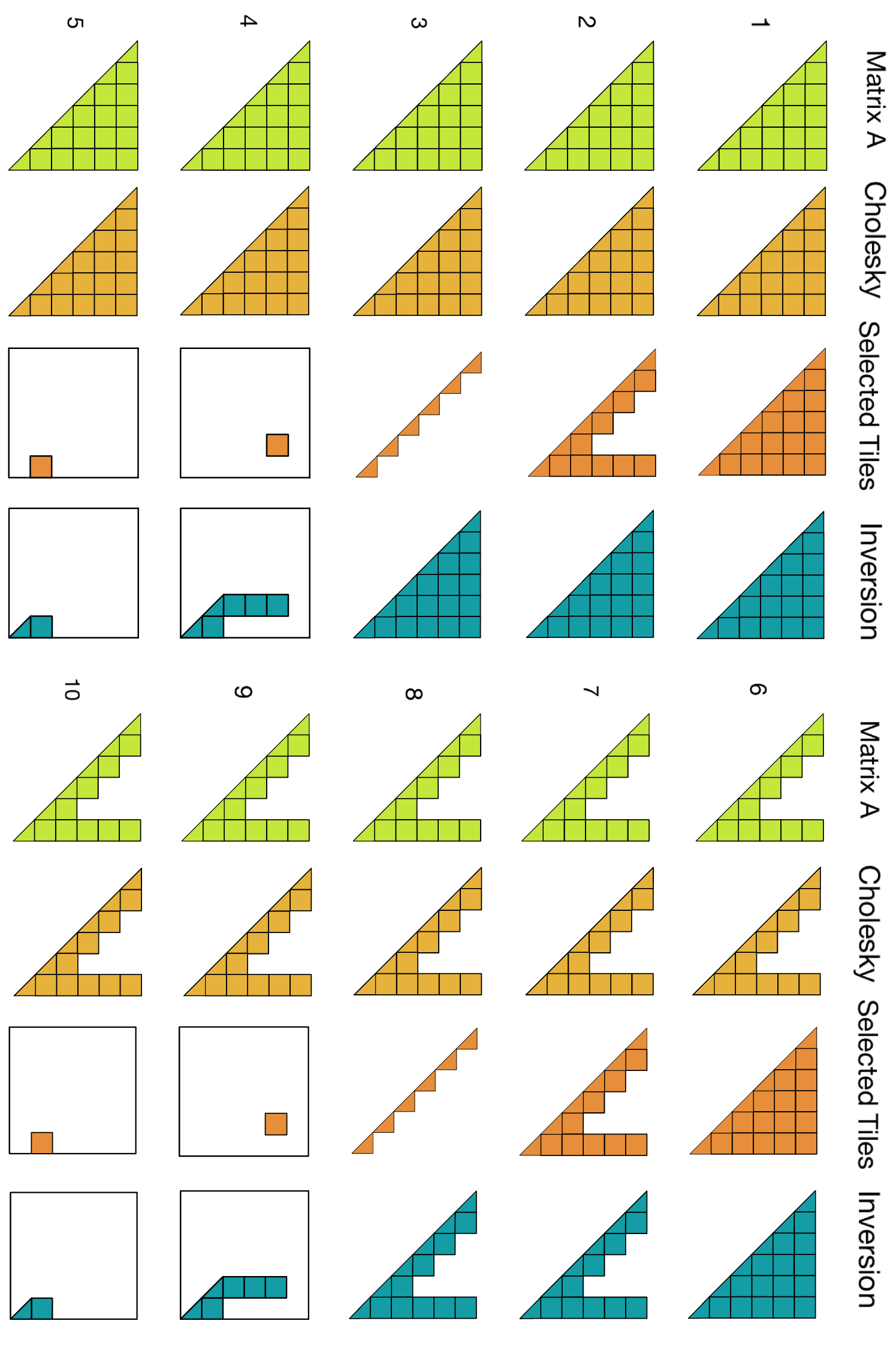
Exposing parallelism in left-looking Cholesky for arrowhead matrices
The Problem: Sequential Bottleneck
In left-looking Cholesky, many GEMMs update the same target tile sequentially:

GEMM → GEMM → GEMM → ... (serial dependency)
The Solution: Tree Reduction
Run GEMMs in parallel to temporary tiles, then combine with tree-based GEADD:
DAG Comparison: Dense vs Arrowhead
6×6 Tiles
Arrowhead structure
Dense Matrix
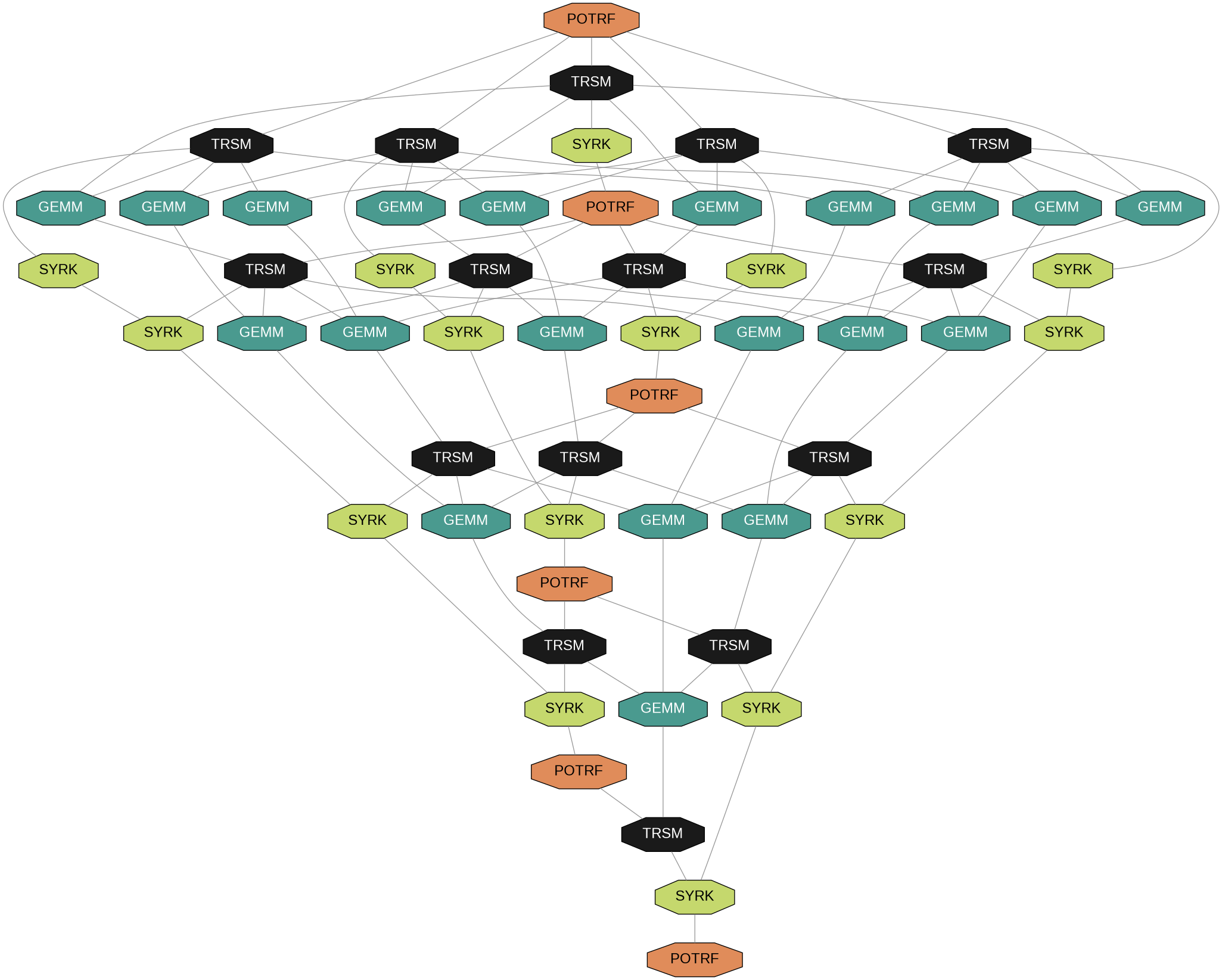
Wide DAG = High parallelism
Arrowhead DAG
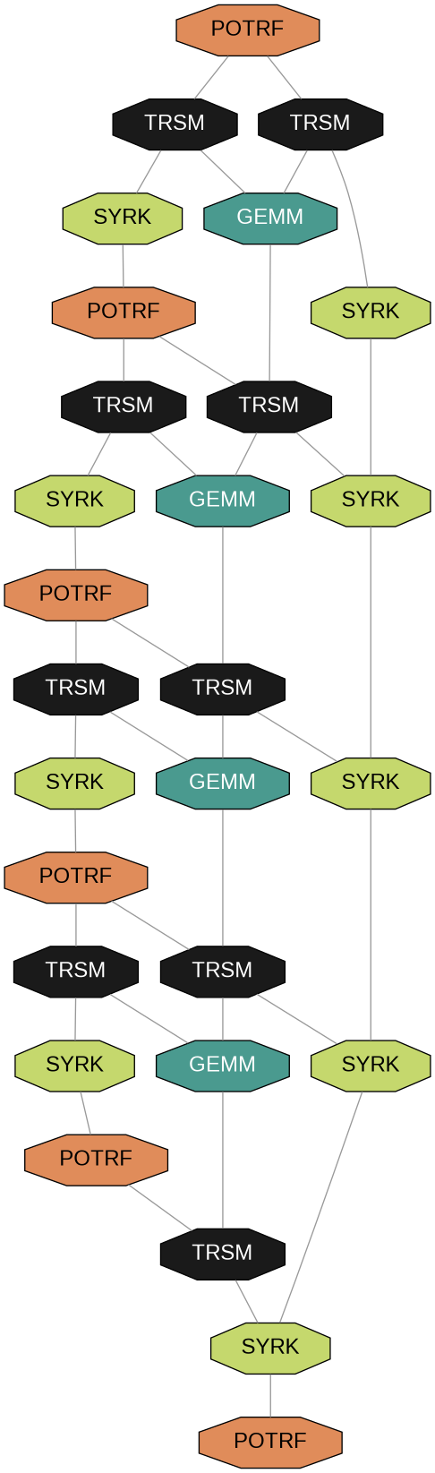
Thin DAG = Limited parallelism
Tree reduction recovers parallelism in the thin arrowhead DAG
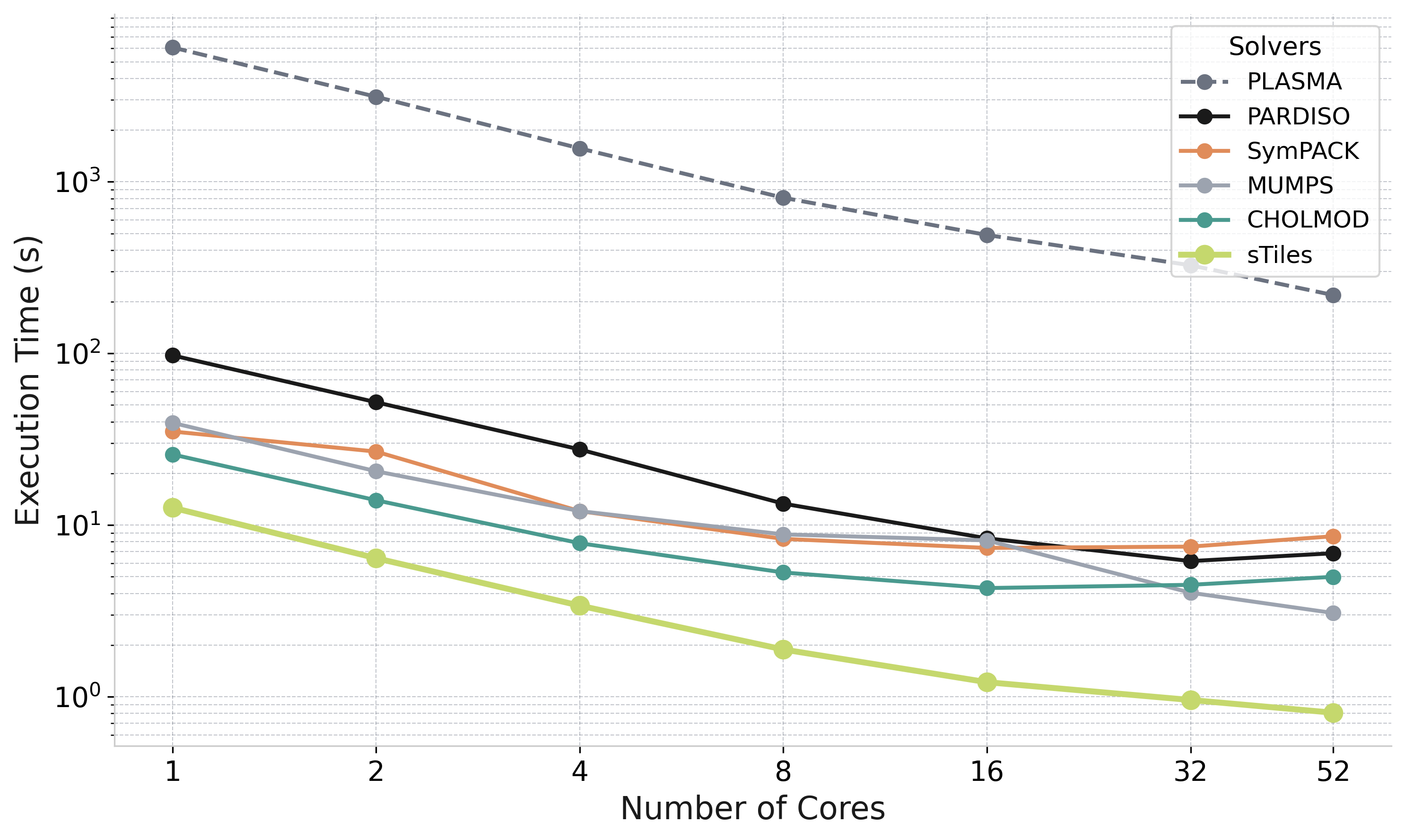
Comparison vs state-of-the-art sparse solvers across 18 test matrices (52 cores)
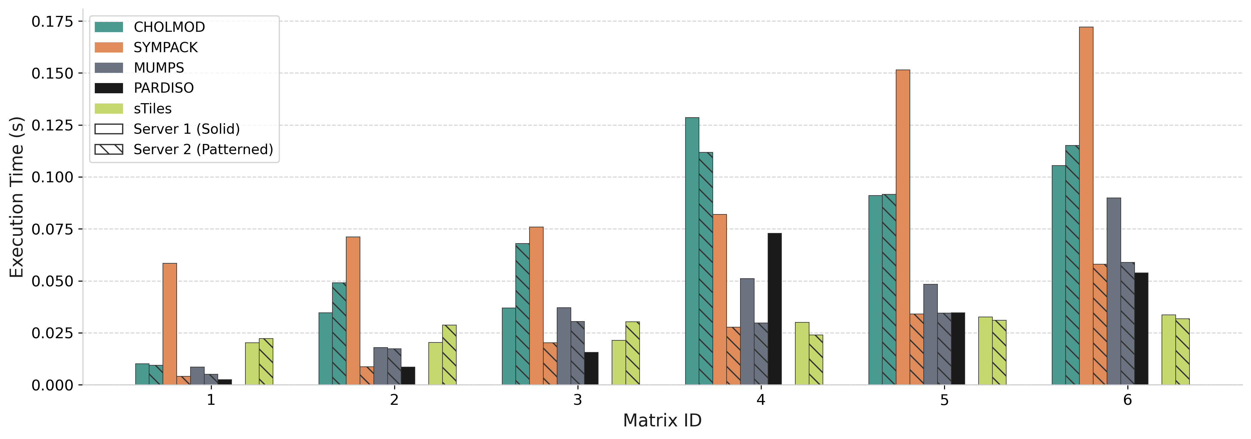
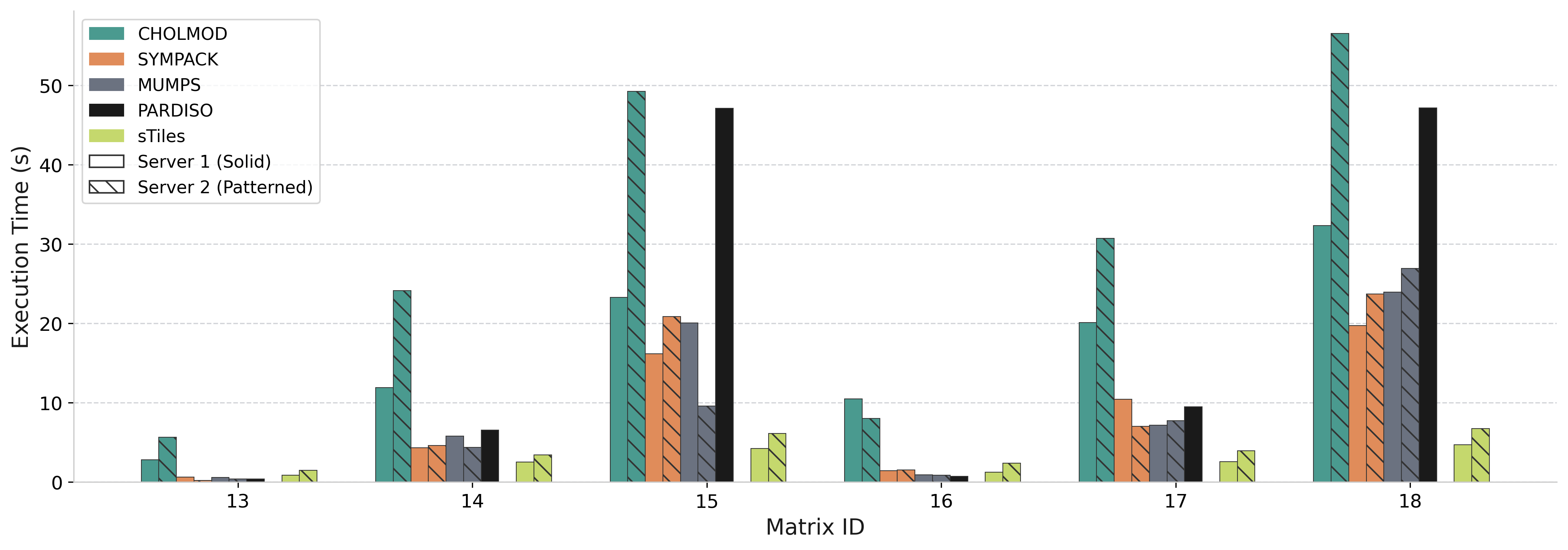
vs PARDISO
0.12× – 11.08×
vs SymPACK
0.72× – 9.34×
vs CHOLMOD
0.50× – 8.41×
vs MUMPS
0.43× – 5.07×
<1× only for narrow BW (≤1000), thin arrowhead
Libraries: CHOLMOD [Chen et al., ACM TOMS 2008], SymPACK [Jacquelin et al., SC 2016], MUMPS [Amestoy et al., 2001], PARDISO [Schenk & Gärtner, 2004]
SuiteSparse matrices : sTiles tiling framework generalizes beyond arrowhead structure
msc23052
n = 23,052 | nnz = 588,933
| Threads | PARDISO (s) | sTiles (s) |
|---|---|---|
| 1 | 0.095 | 0.658 |
| 8 | 0.031 | 0.112 |
| 16 | 0.028 | 0.078 |
| 32 | 0.035 | 0.076 |
| 52 | 0.042 | 0.113 |
ship_001
n = 34,920 | nnz = 3,896,496
| Threads | PARDISO (s) | sTiles (s) |
|---|---|---|
| 1 | 0.393 | 0.591 |
| 8 | 0.080 | 0.104 |
| 16 | 0.077 | 0.077 |
| 32 | 0.064 | 0.089 |
| 50 | 0.079 | 0.088 |
nd6k
n = 18,000 | nnz = 6,897,316
| Threads | PARDISO (s) | sTiles (s) |
|---|---|---|
| 1 | 5.335 | 3.479 |
| 8 | 0.849 | 0.540 |
| 16 | 0.550 | 0.351 |
| 32 | 0.483 | 0.409 |
| 52 | 0.552 | 0.456 |
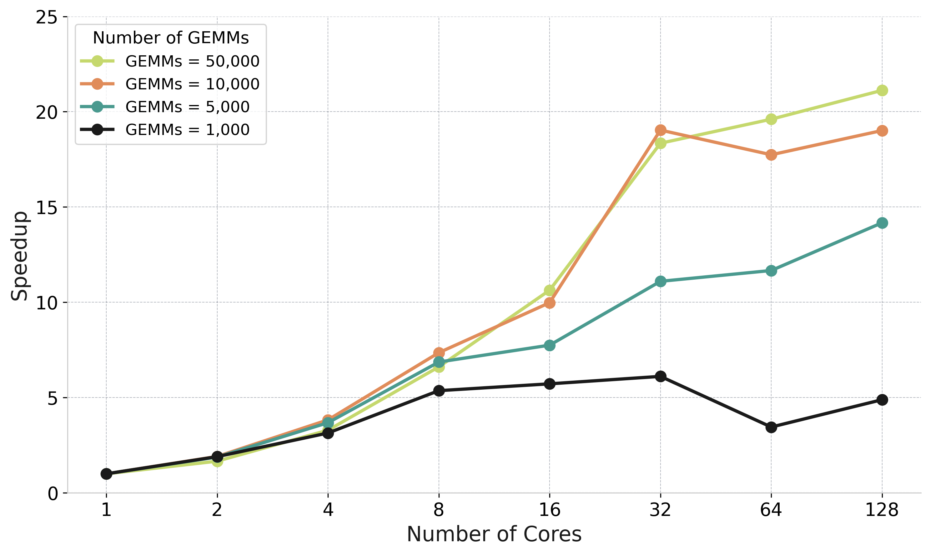
Parallel GEMM accumulation: speedup from tree reduction vs sequential
The Problem
Left-looking Cholesky: many GEMMs update same target tile sequentially
Tree Reduction Solution
Parallel GEMMs to temporary tiles → Tree-based GEADD accumulation → Final update
Speedup up to
5× at 16-32 cores
50K
GEMMs benefit most
log₂(n)
Reduction depth
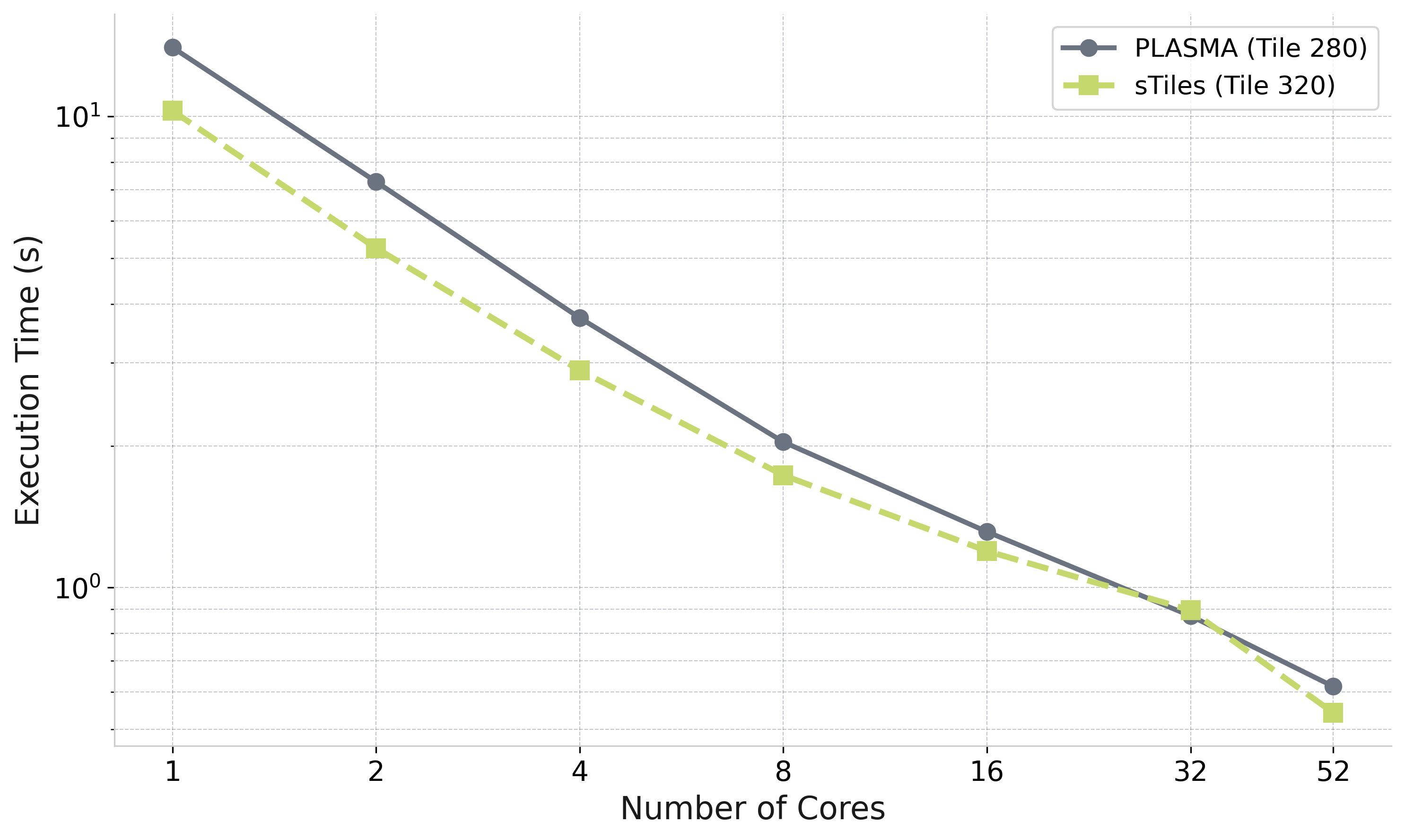
Strong scaling: Matrix 9 (n=100K, BW=3000, thick=10) — Intel Xeon 6230R, 1 to 52 cores
sTiles parallel efficiency (this matrix)
| 1 → 8 cores | 84% |
| 1 → 16 cores | 65% |
| 1 → 32 cores | 41% |
| 1 → 52 cores | 30% |
Efficiency drops beyond 16 cores
The arrowhead structure has a long critical path — available parallelism is bounded regardless of core count
PLASMA included as reference
Illustrates the cost of ignoring sparsity — not a practical competitor for this problem class
More details on this in my talk at:
Friday, March 6 : CP12 : 11:15–11:35 AM : Room T9 SR 055
GPU-Accelerated Parallel Selected Inversion for Structured Matrices
Esmail Abdul Fattah, Hatem Ltaief, Haavard Rue, David E. Keyes : KAUST
Goal: compute A−1ij for all (i,j) in the sparsity pattern of A, not just a few entries
Non-zeros of A
(before fill-in)
→
compute A−1ij
at every (i,j)
where Aij ≠ 0
Selected entries of A−1

(same sparsity pattern)
MUMPS
Solves A·x = eᵢ per entry via elimination tree pruning. Efficient for few arbitrary entries, not for computing the full sparsity pattern.
Amestoy et al., SIAM J. Matrix Anal. Appl., 2001
PSelInv (PEXSI)
Supernodal left-looking selected inversion. Slower than PARDISO on large structured problems, with out-of-memory failures. PEXSI is not actively maintained.
Jacquelin et al., ACM TOMS, 2017 | Verbosio, PhD thesis, 2019
Serinv
Specialized for block-tridiagonal + arrowhead matrices only. sTiles targets general sparse SPD matrices beyond this fixed structure.
Maillou et al., arXiv:2503.17528, 2025
Panua-PARDISO ✓ chosen benchmark
State-of-the-art supernodal LLT solver, strongest competitor for full-pattern selected inversion.
Schenk et al., Future Gener. Comput. Syst., 2001 | Schenk & Gärtner, Parallel Comput., 2002
sTiles vs PARDISO for selected inversion on 500K matrices (computing (A⁻¹)ᵢⱼ on sparsity pattern)
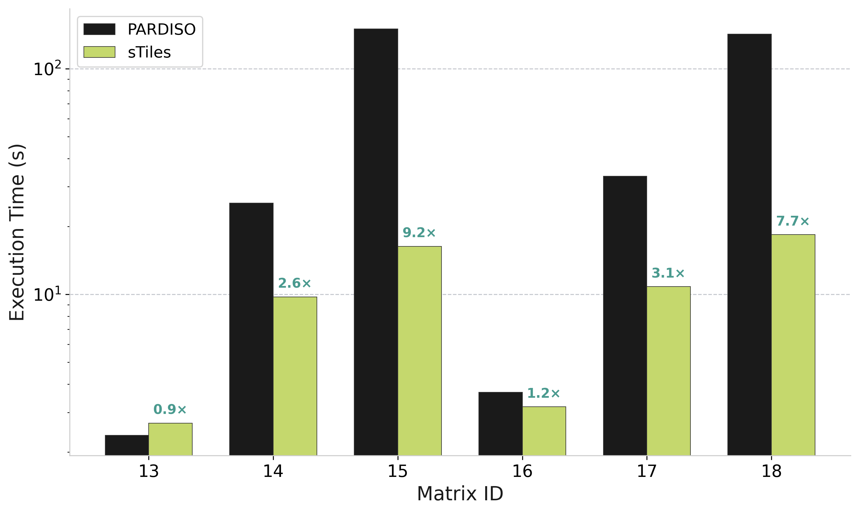
Speedup vs PARDISO
0.9× – 9.2×
Matrix 15 (n=500K, b=3000)
High Bandwidth Matrices
IDs 14, 15, 17, 18: 2.6× to 9.2× faster than PARDISO
Low Bandwidth Matrices
IDs 13, 16: Similar performance (sparse overhead dominates)
When sTiles Wins
High-bandwidth matrices: dense tiles enable BLAS efficiency : advantage grows with bandwidth
Reference: PARDISO Selected Inversion [Schenk et al., SIAM SISC 2007]
How inverse time scales with matrix density (100K matrices | Set 1: BW=1500, Set 2: BW=3000)
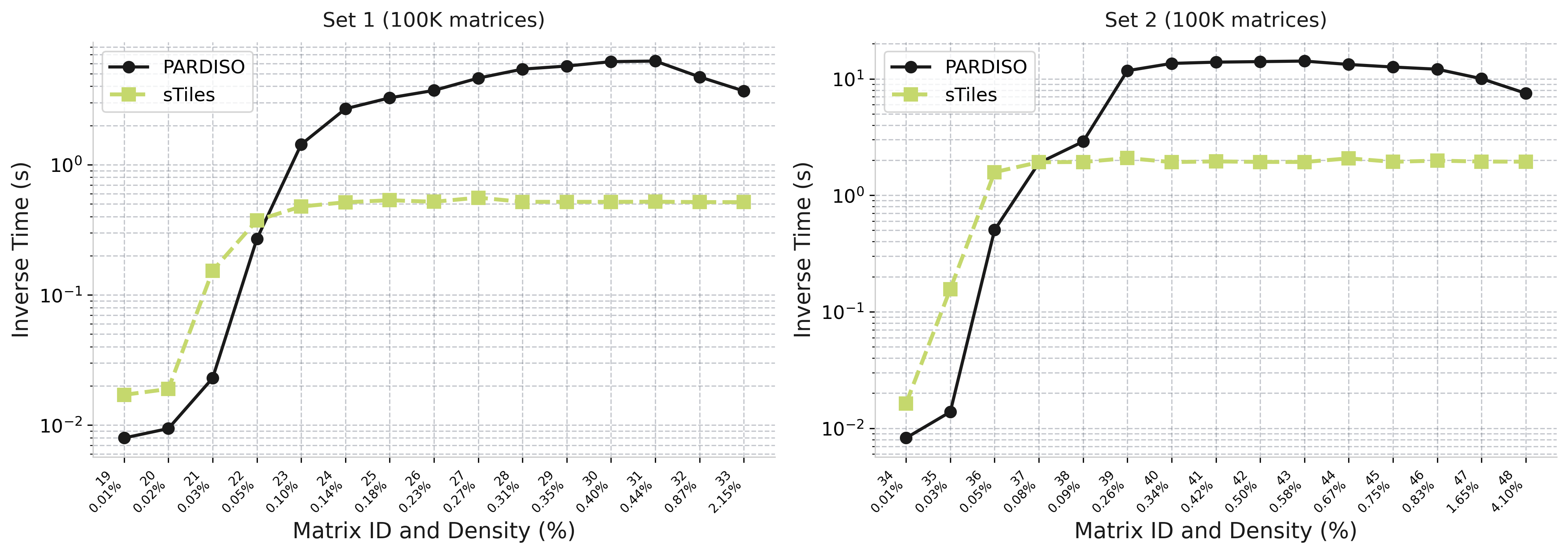
sTiles (lime)
Flat scaling - time stays constant as density increases
PARDISO (black)
Growing cost - time increases with density
Why sTiles stays flat:
Fixed tile size → predictable BLAS workload
0.15× – 12×
Speedup range (Set 1)
0.09× – 7.4×
Speedup range (Set 2)
One matrix (n=10,200, fully dense) — static vs dynamic scheduling — not a general claim
Observation (this matrix)
sTiles and PLASMA track closely across all core counts
PLASMA: Parallel Linear Algebra Software for Multicore Architectures [Agullo et al., 2009]