What's Slowing Down Your Statistical Model, and How Tiling Fixes It?
Esmail Abdul Fattah
King Abdullah University of Science and Technology (KAUST)
Seminar Talk, Cirad, Montpellier, France · April 2026
Bayesian models for spatial, temporal, and hierarchical data are becoming increasingly complex. Yet the computational cost often forces researchers to simplify. In this talk:
Where the bottleneck comes from
Why existing solvers struggle with statistical matrix structures
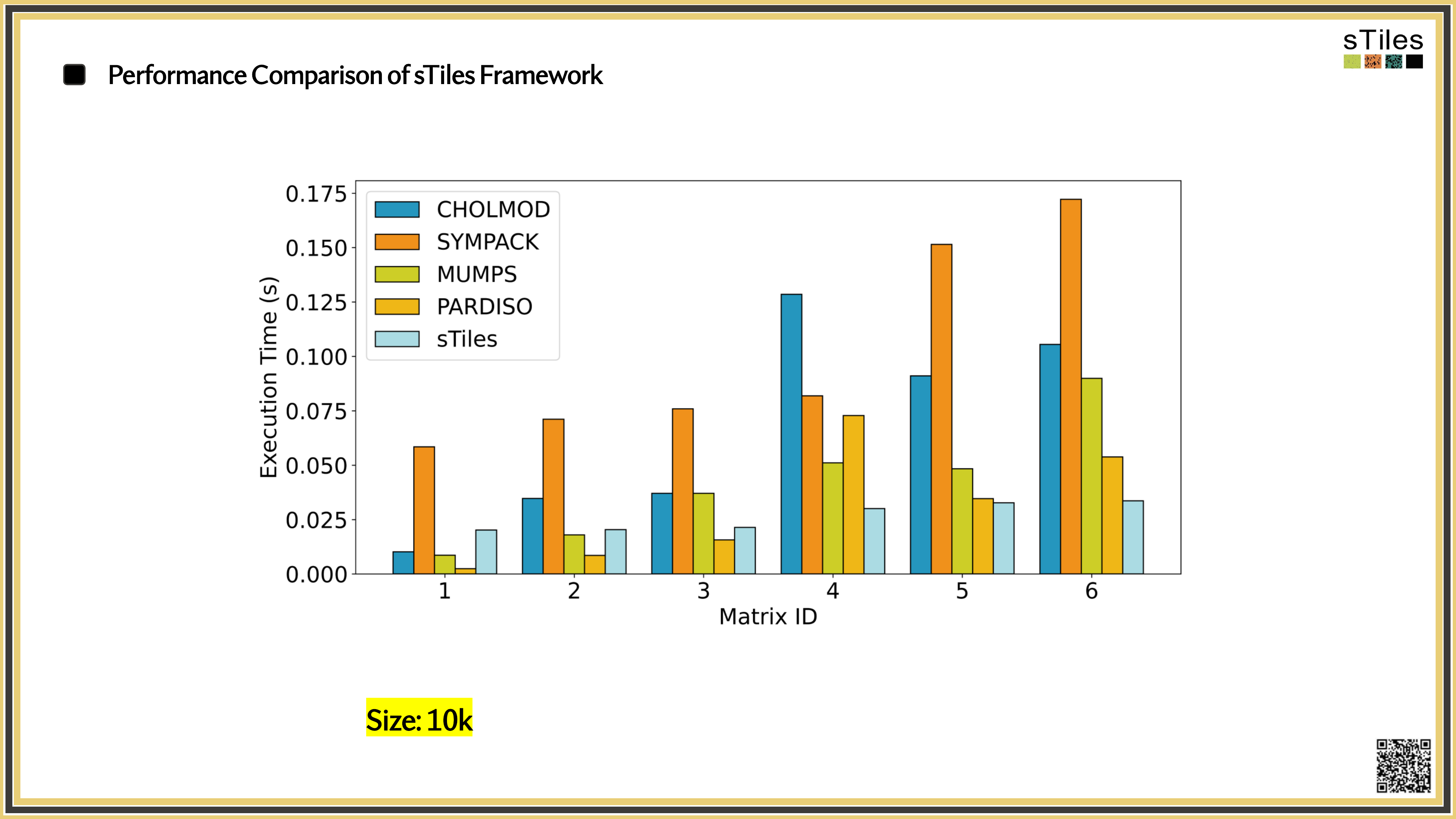
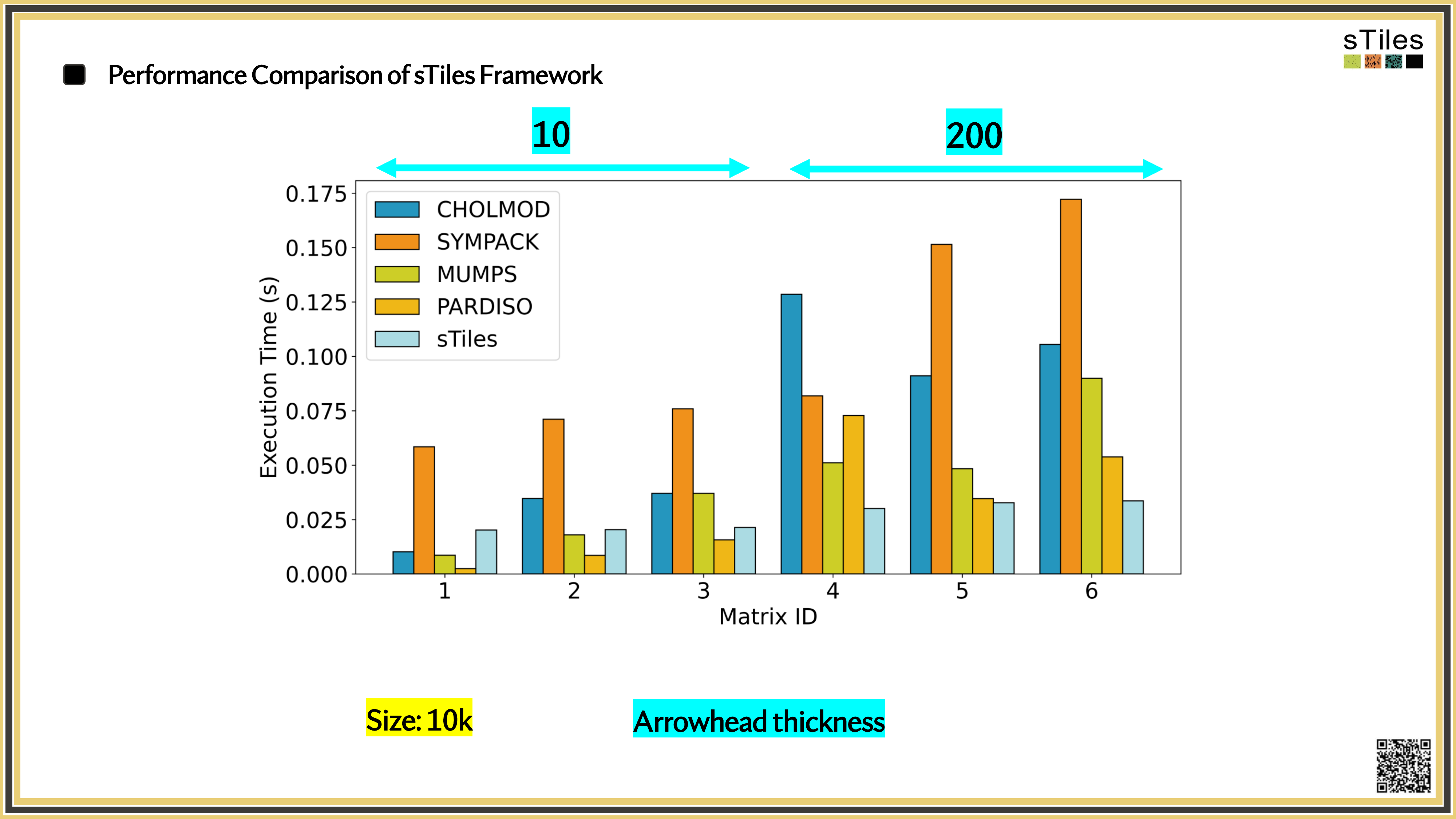
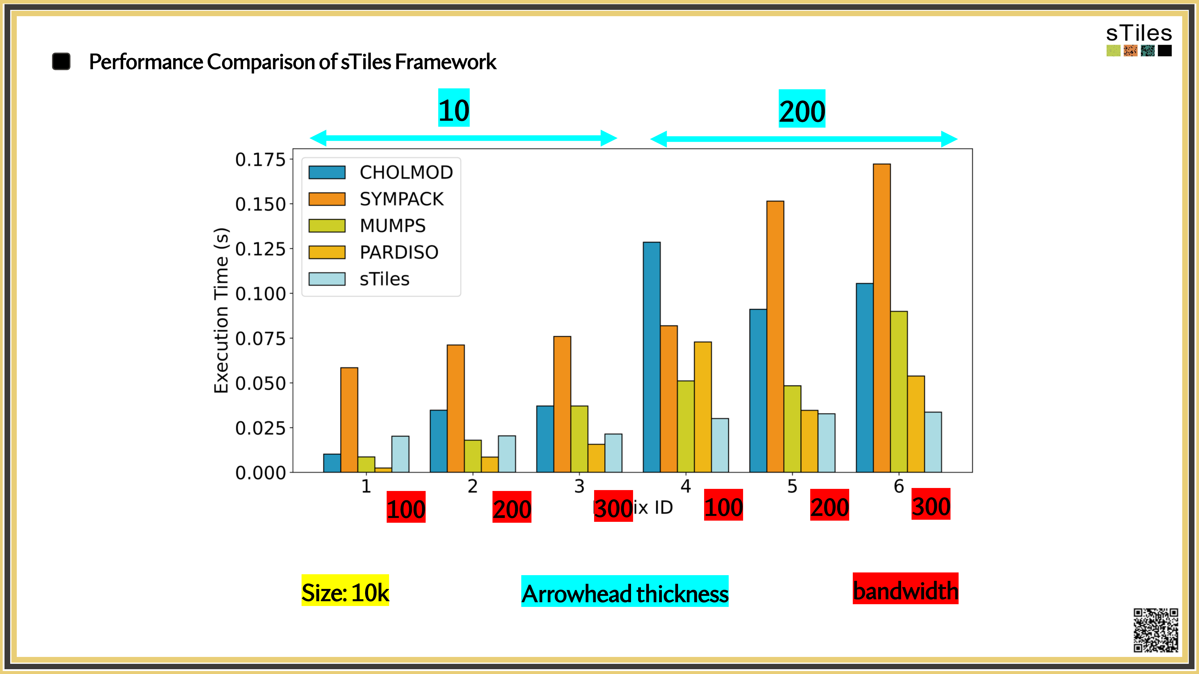
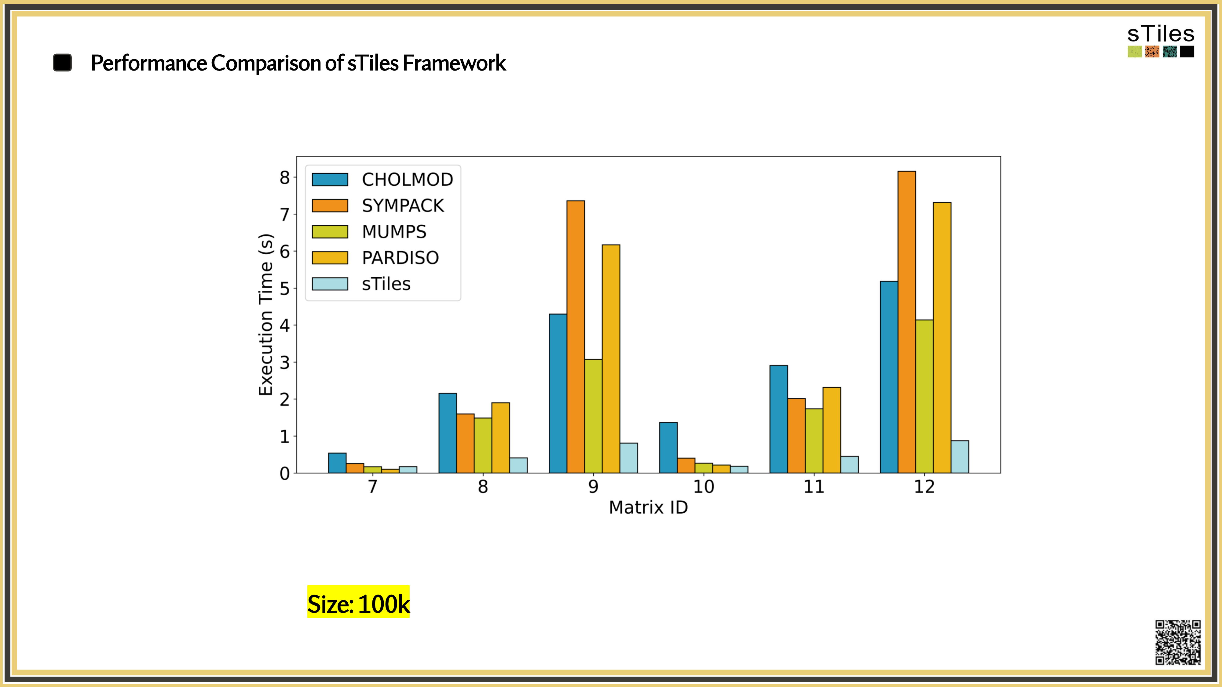
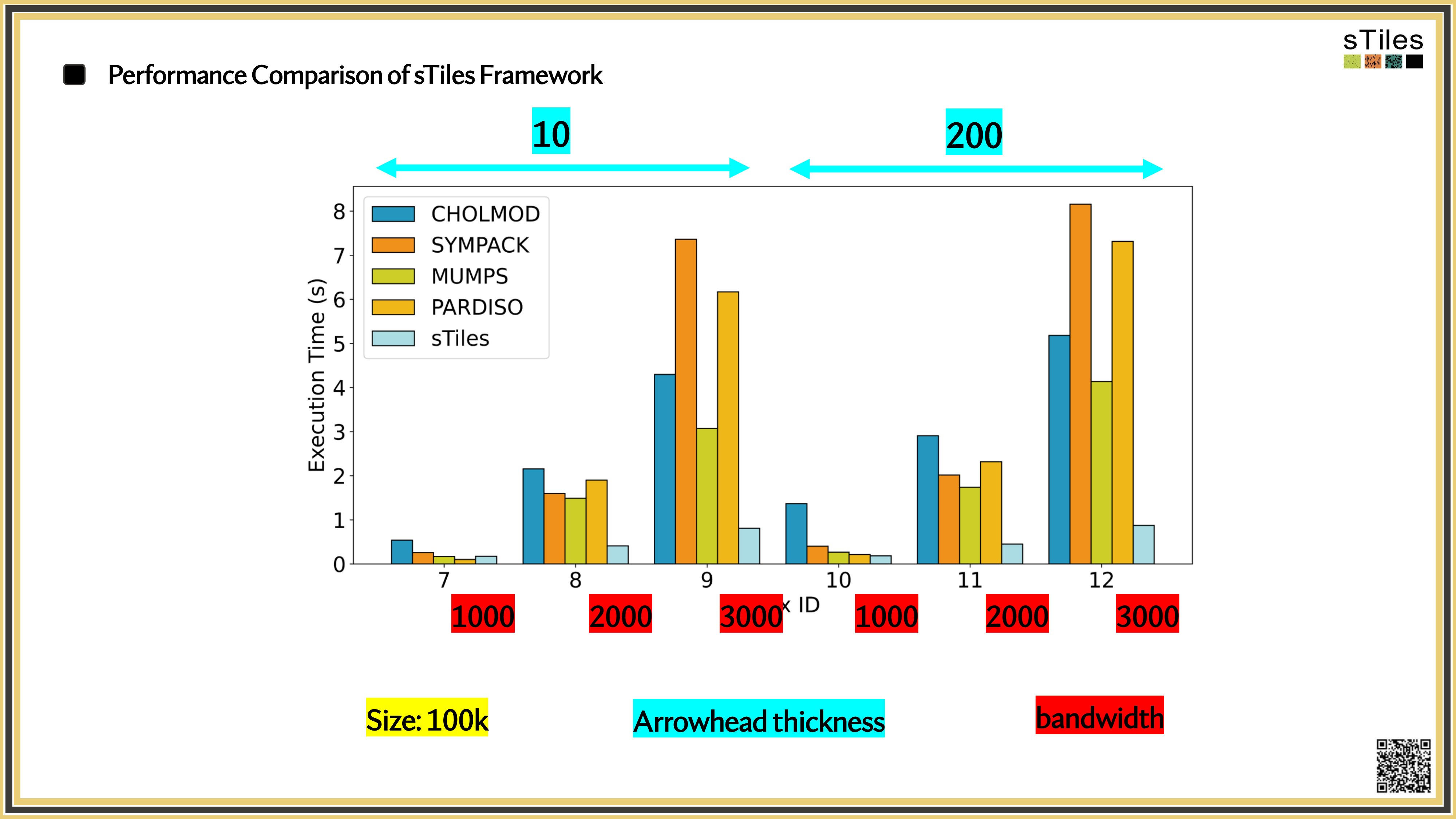
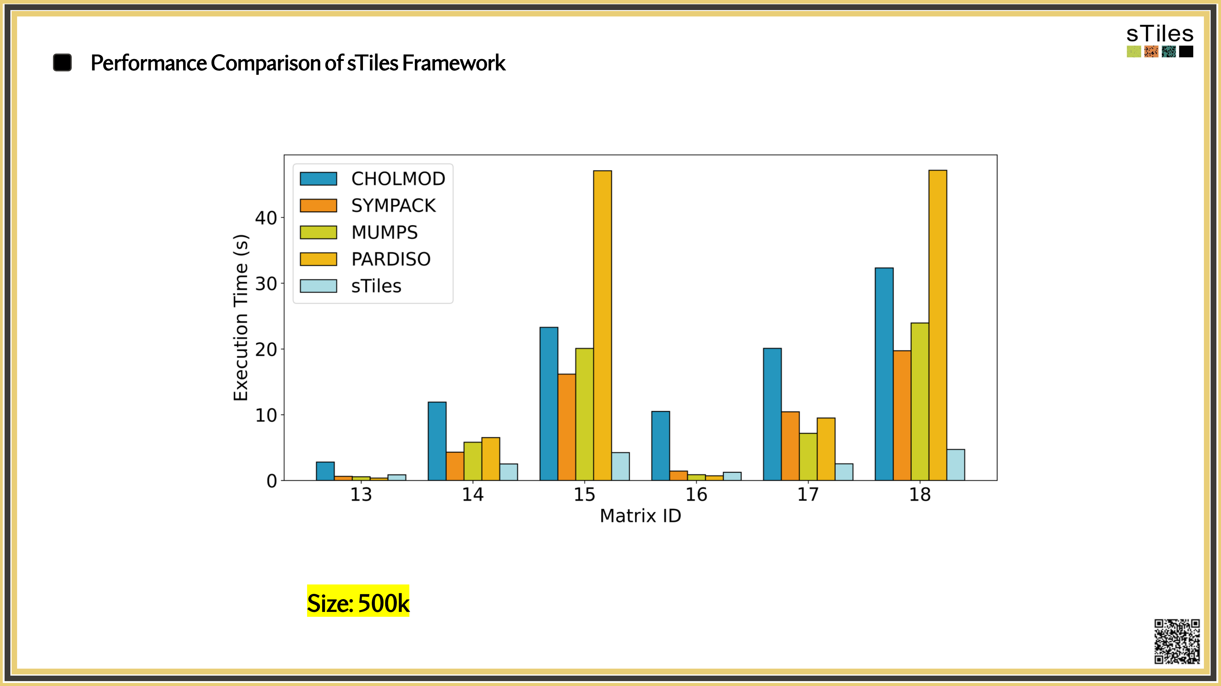
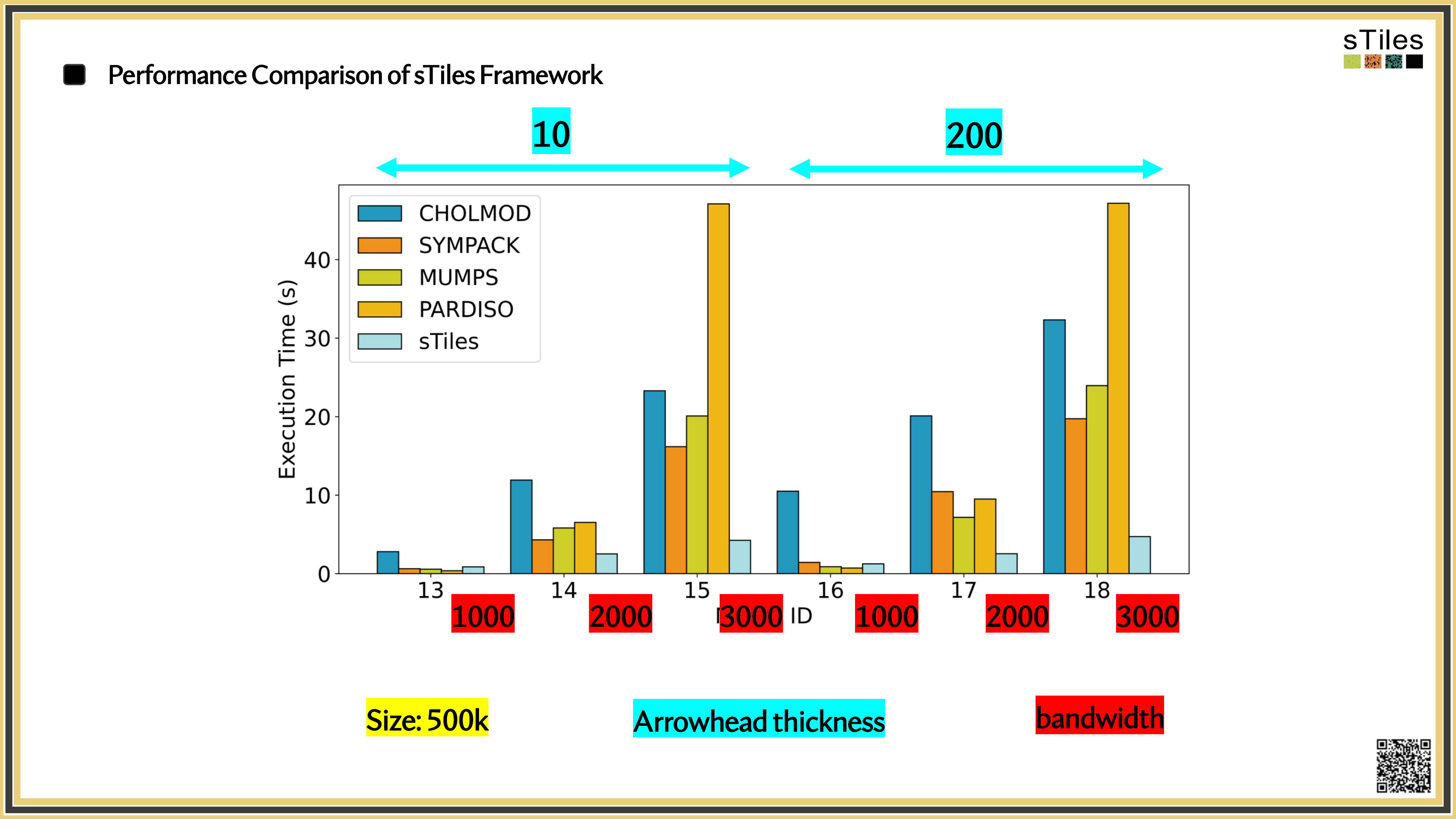
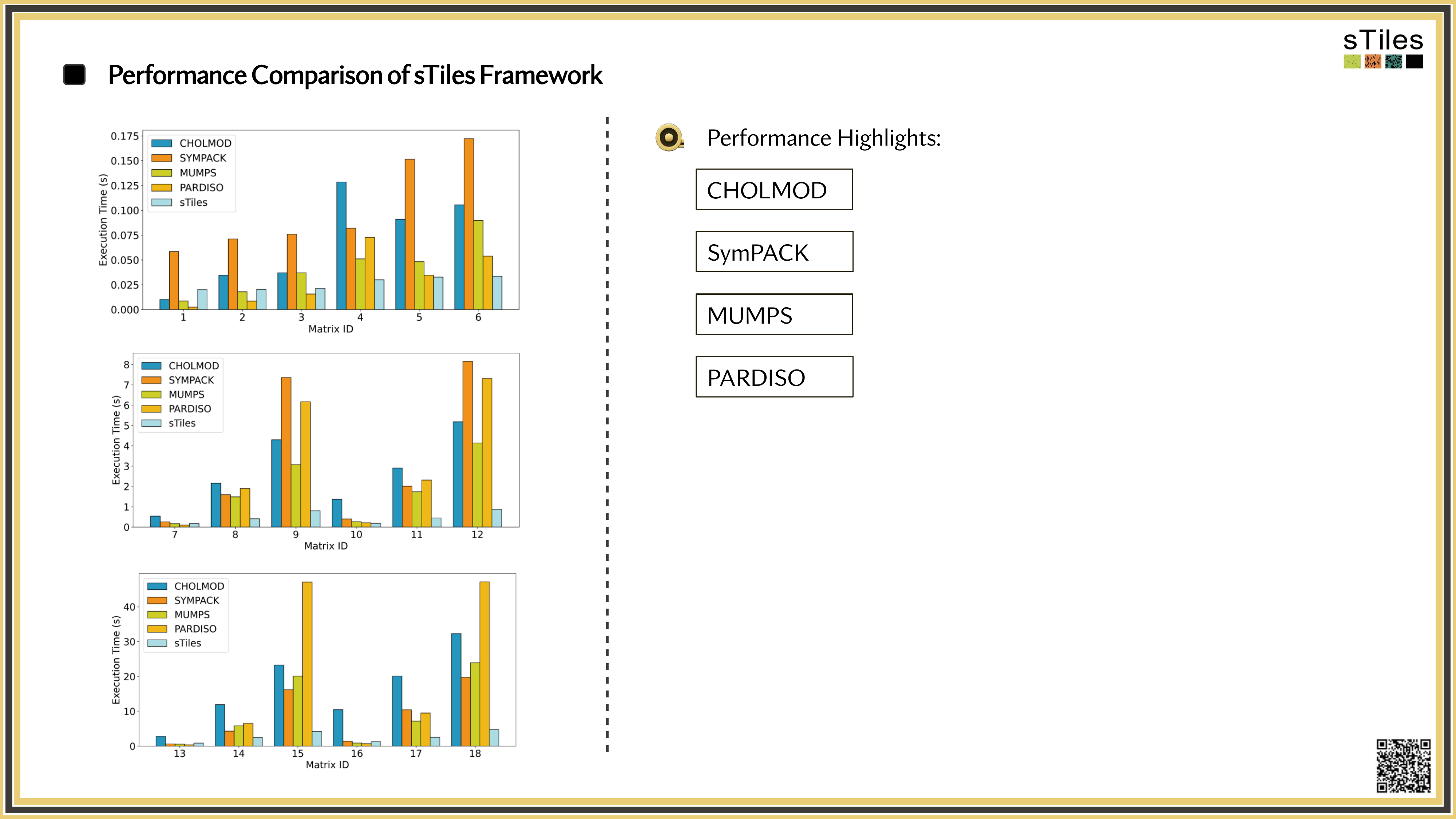
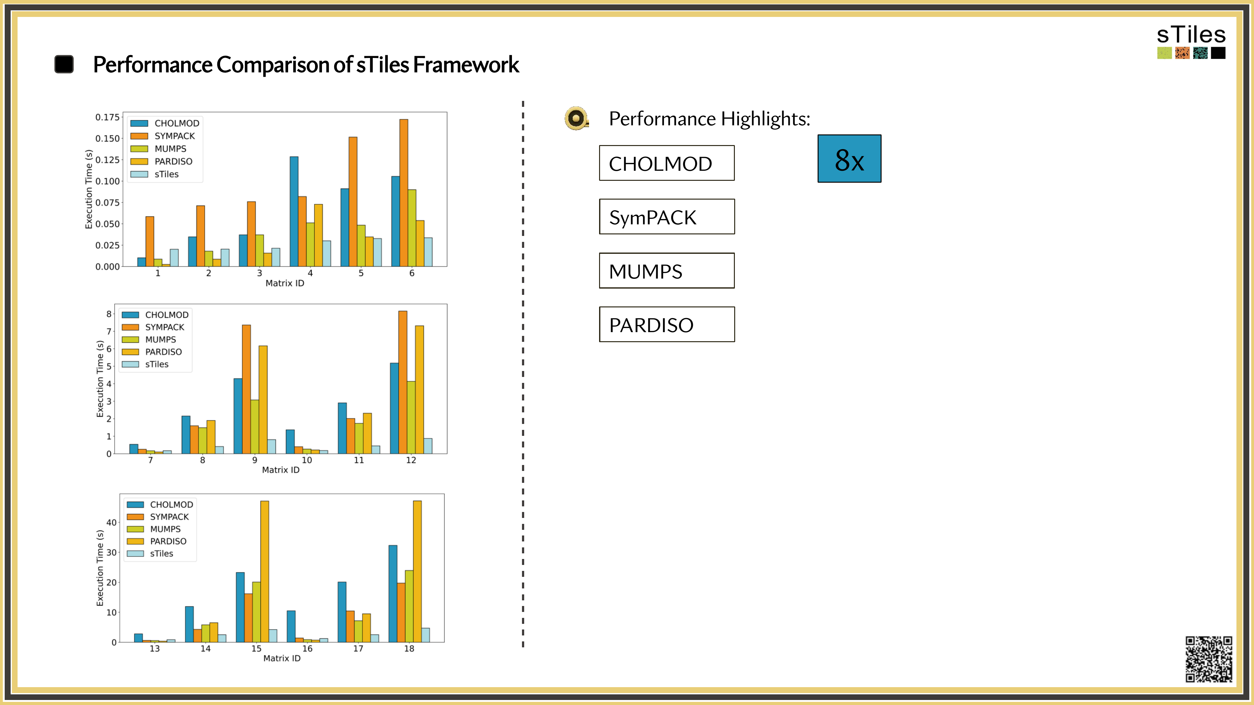
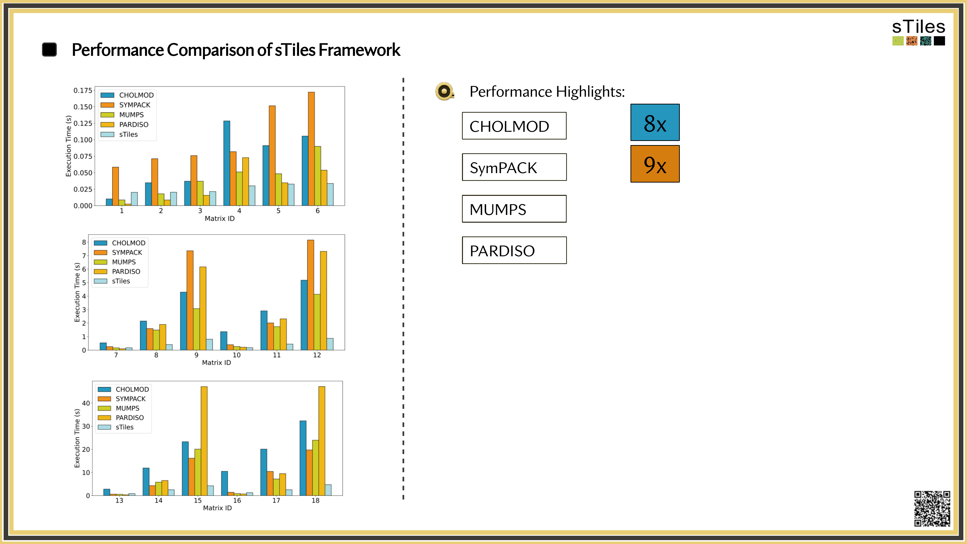
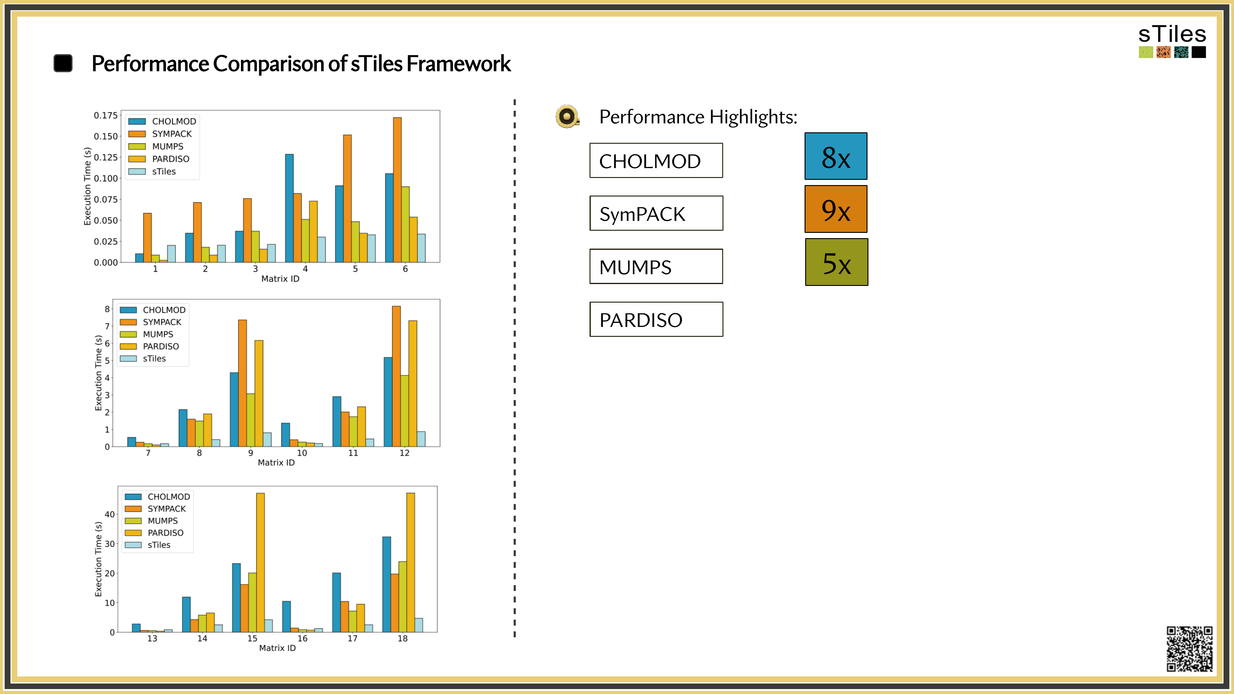
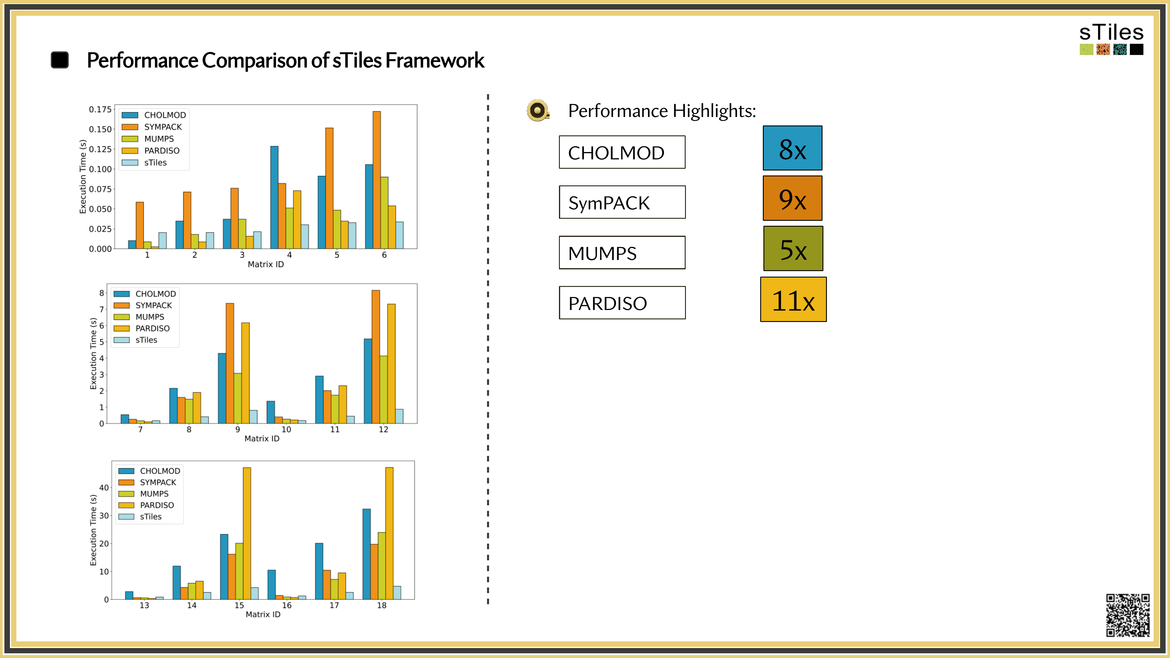
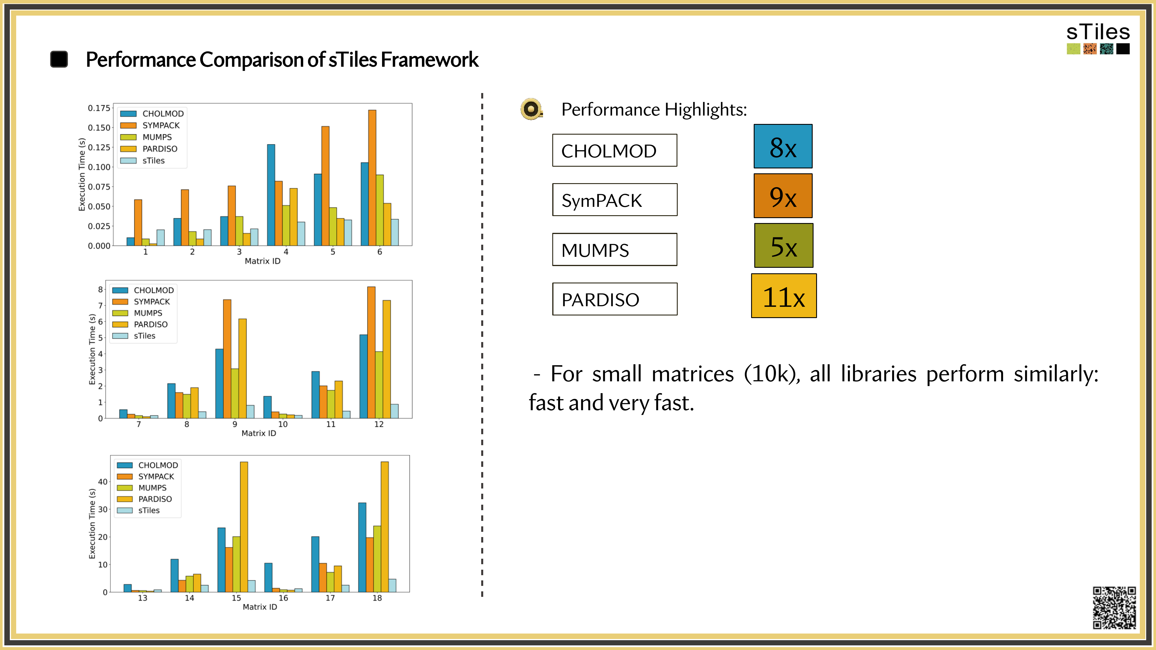
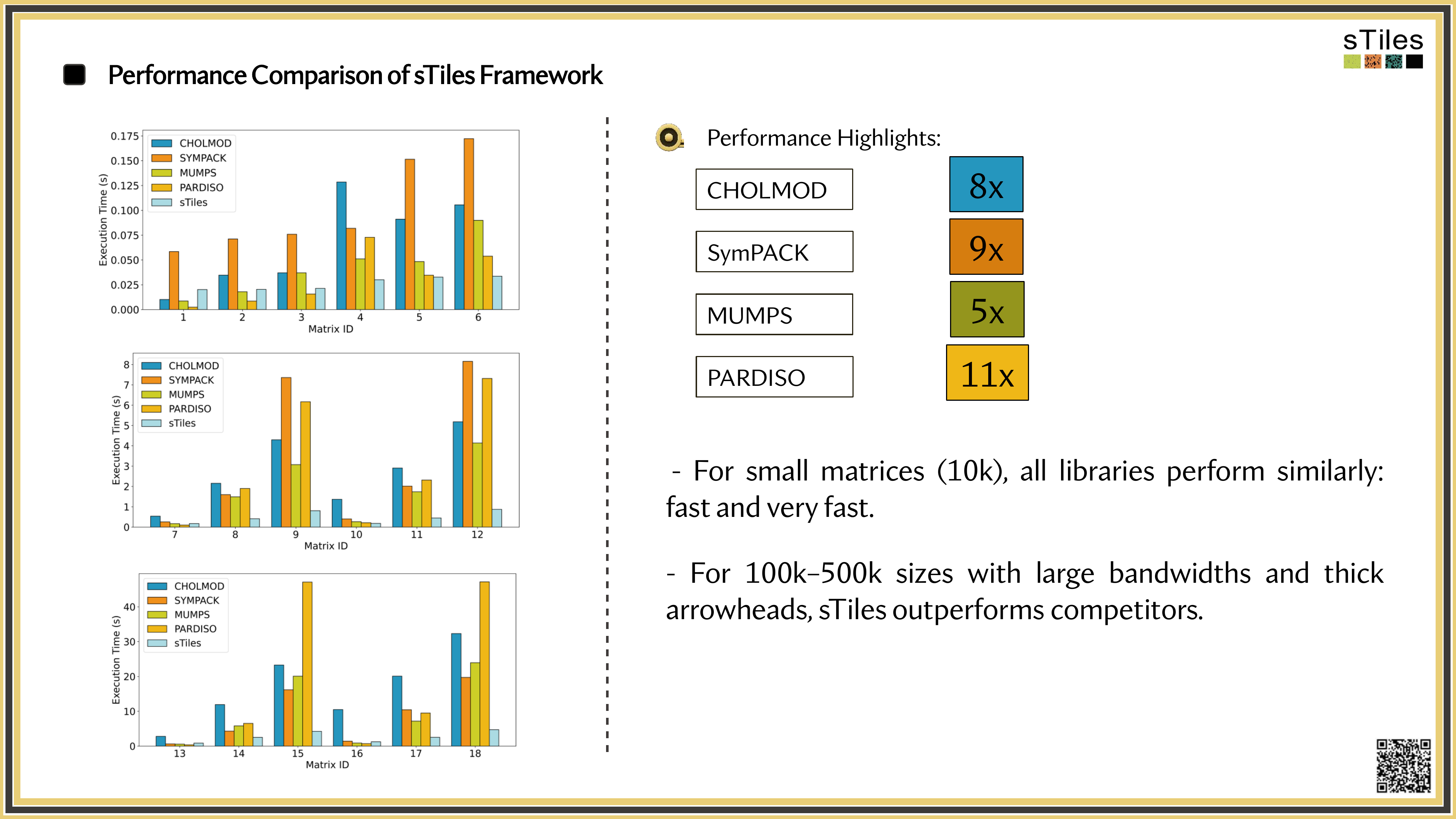
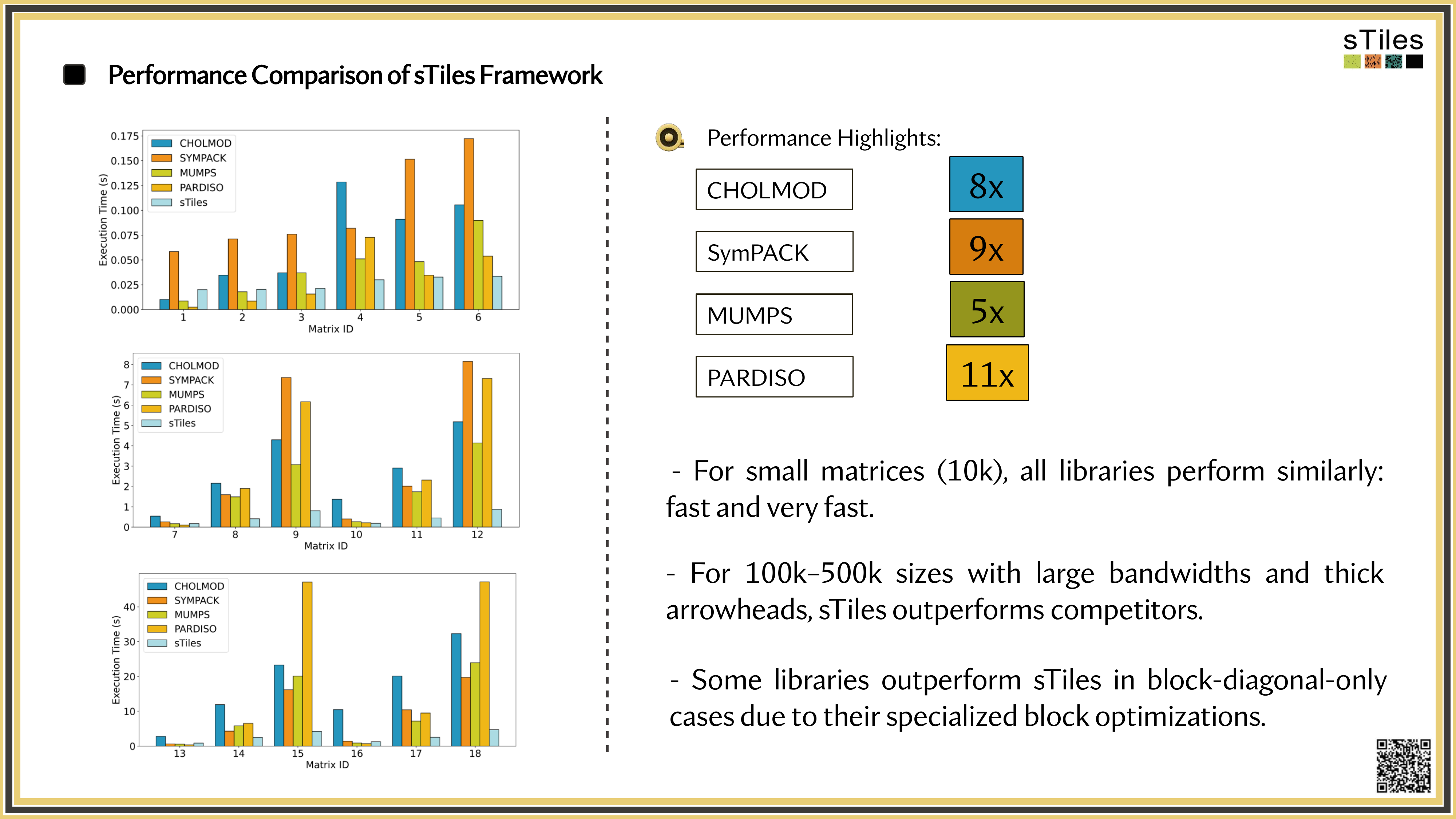
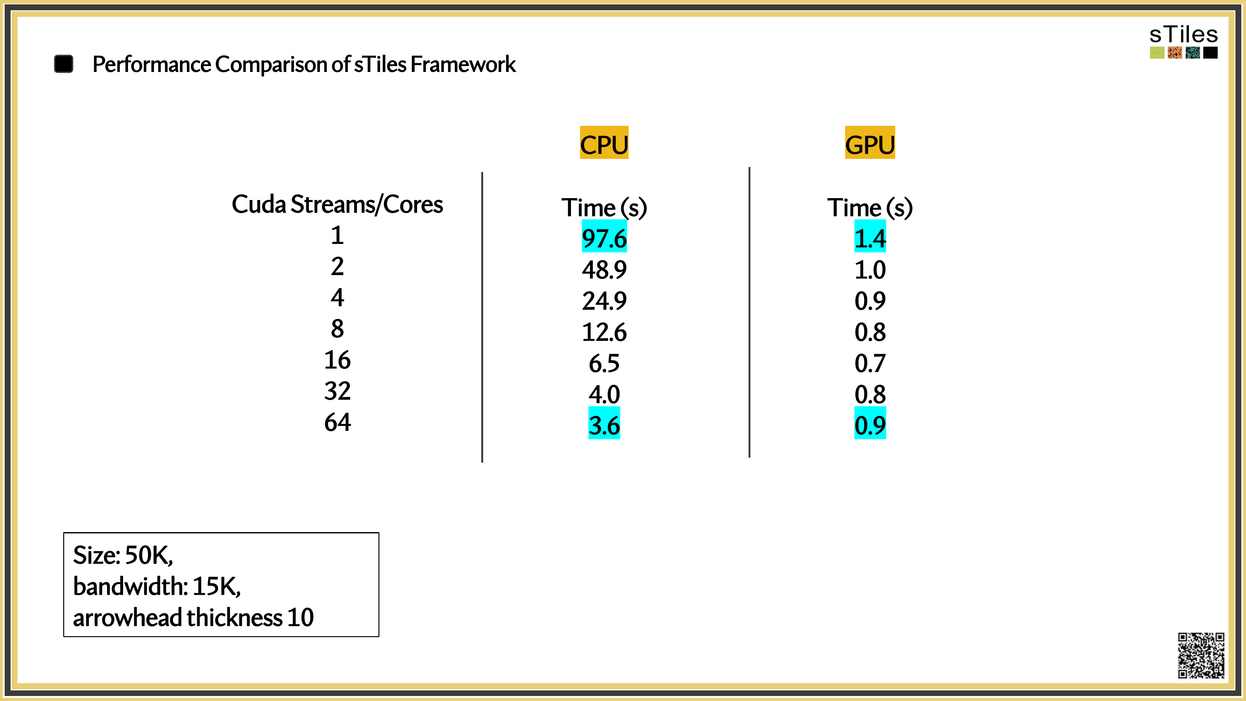
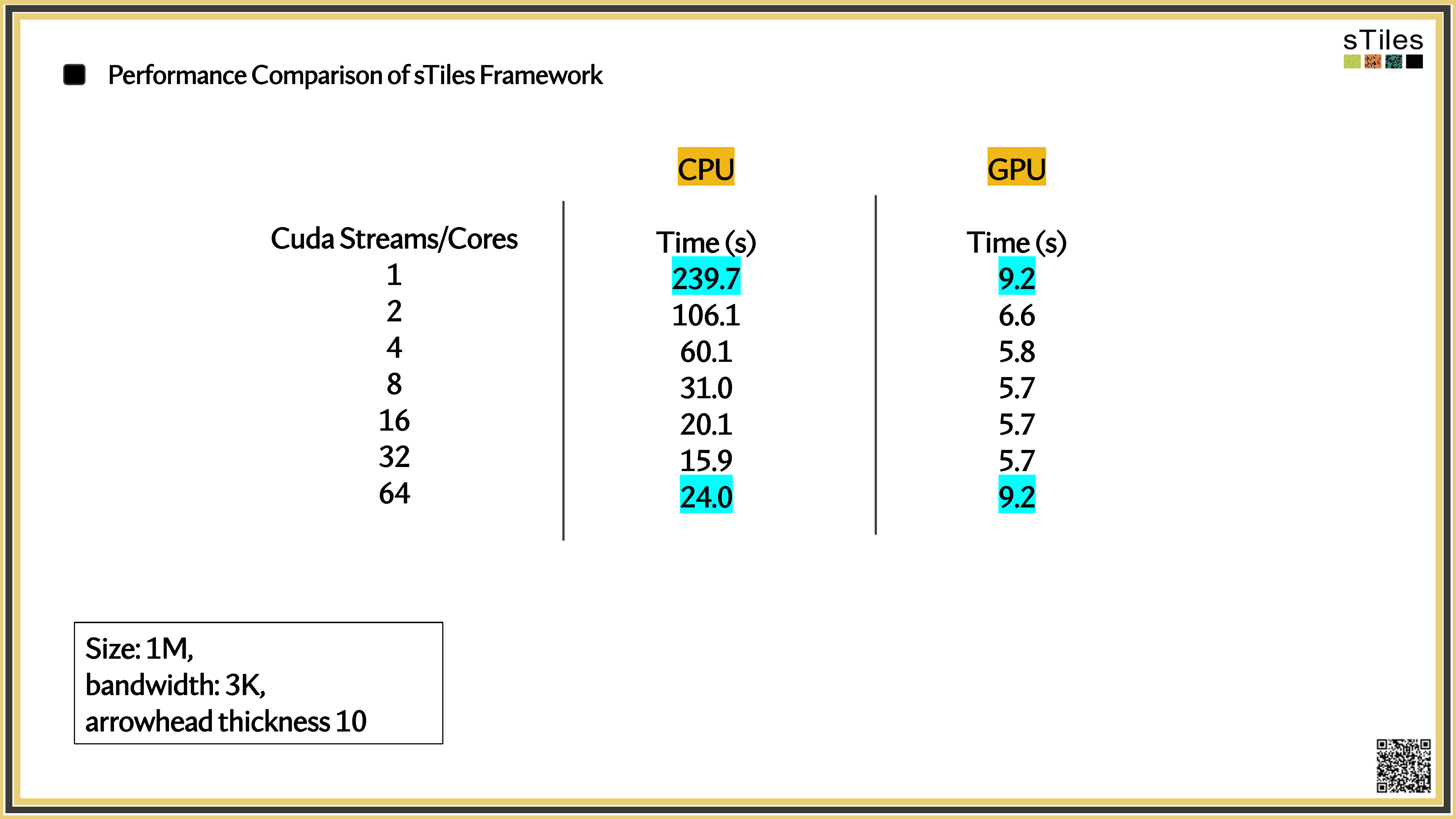
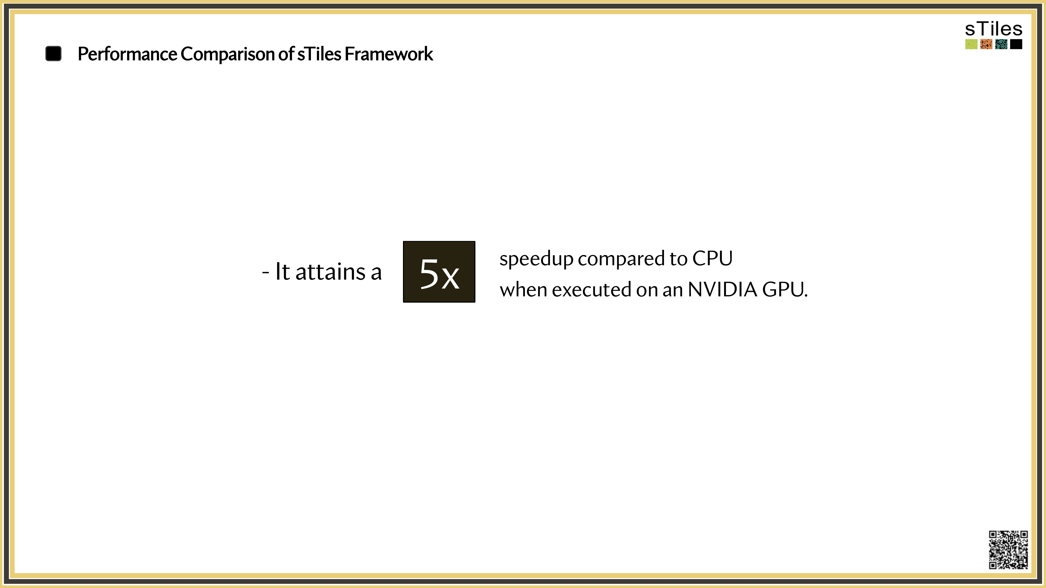
How sTiles exploits internal structure for up to 11x speedups
The goal: fit the model you want, not the model your hardware allows.
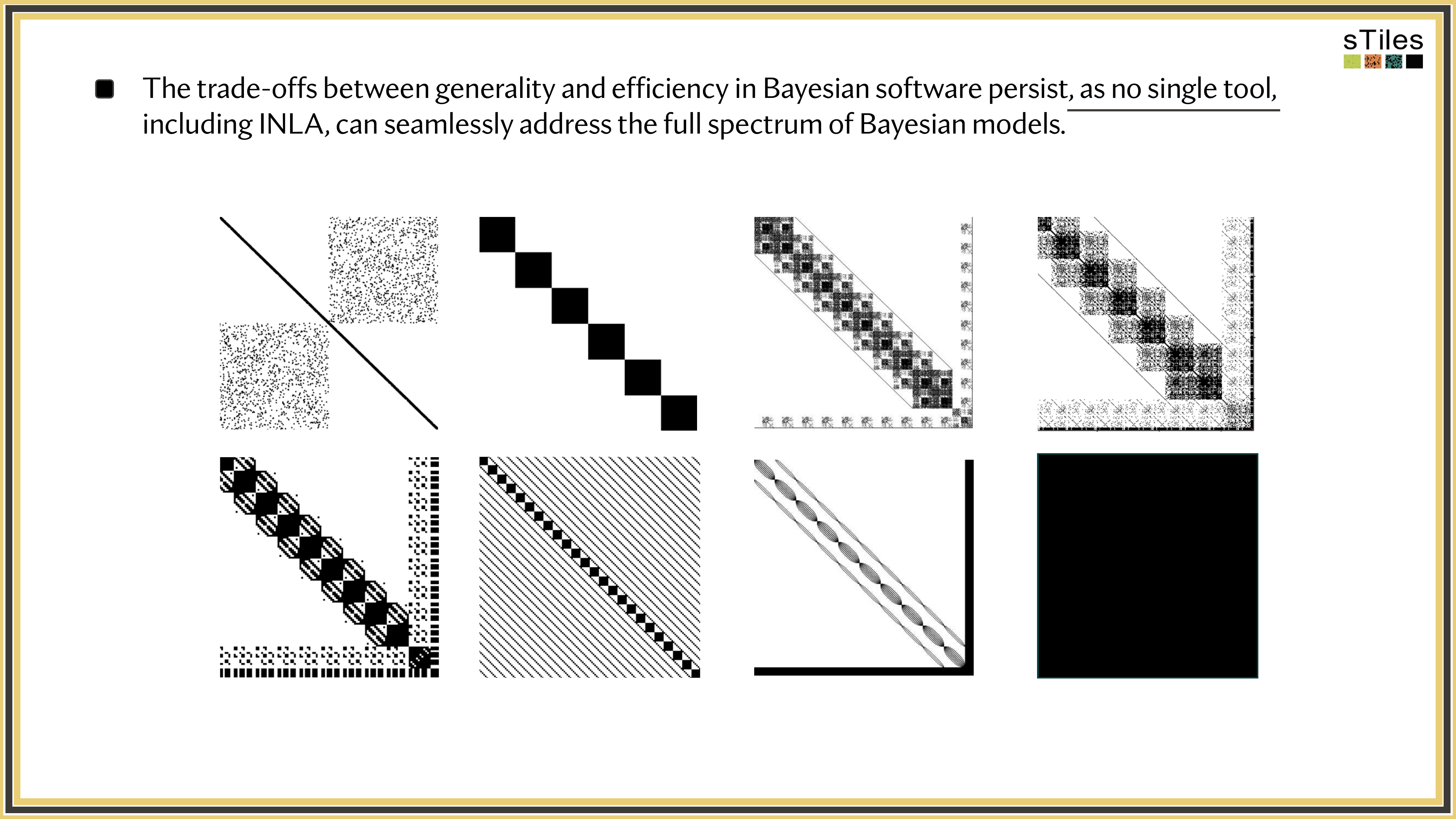
Stan, TMB, INLA, GPs. Different tools, same wall.
And as models grow, we all simplify the same way: coarser grids, fewer random effects, dropped interactions.
What does your computer actually do?
When you fit a mixed, spatial, or Bayesian model, the software builds a matrix A from your model and asks:
A · x = b
"Find the x that makes this true."
Every posterior, every likelihood, every iteration goes through this.
If solving A · x = b is slow, your model is slow.
We have two ways to solve it.
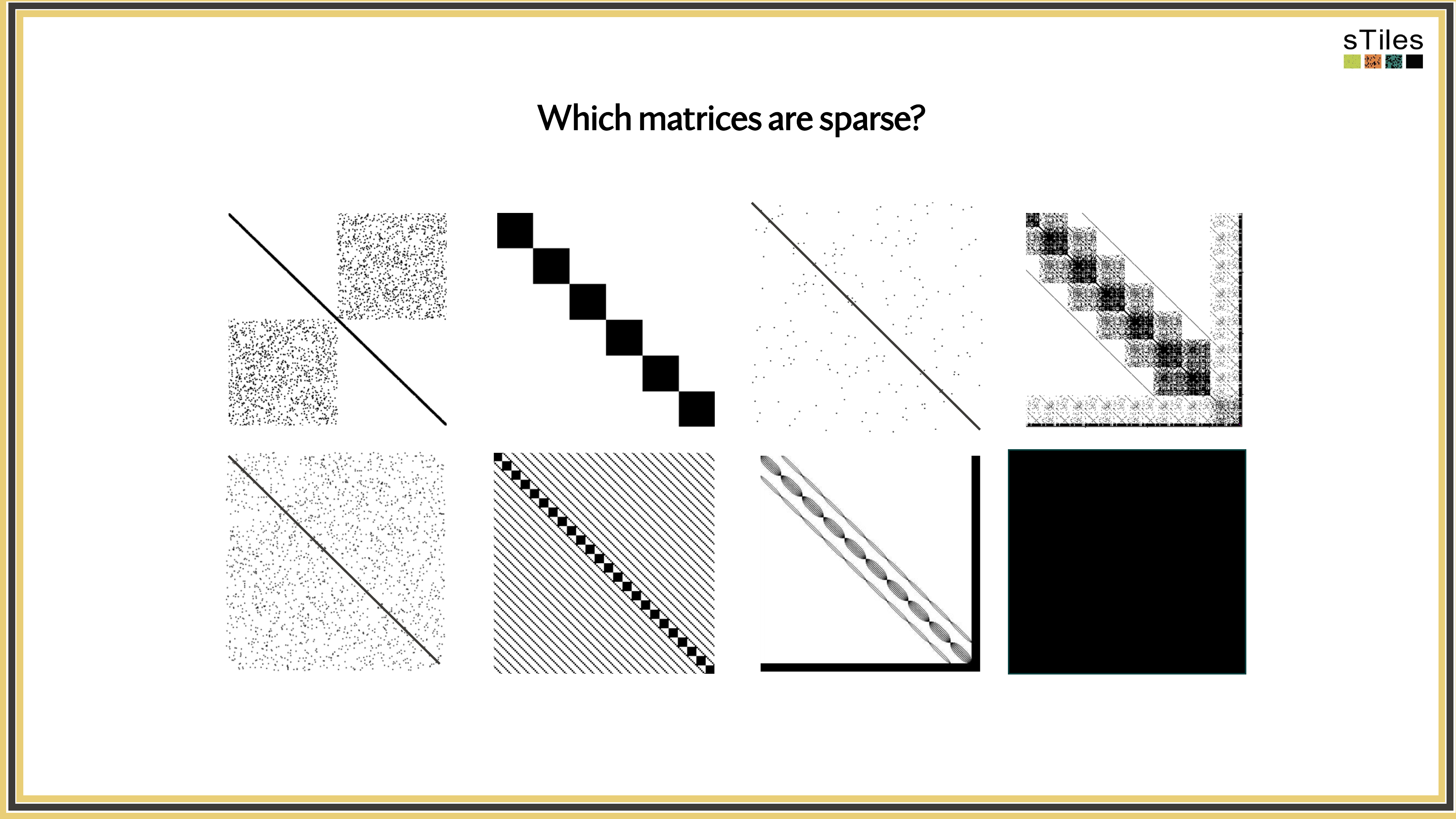
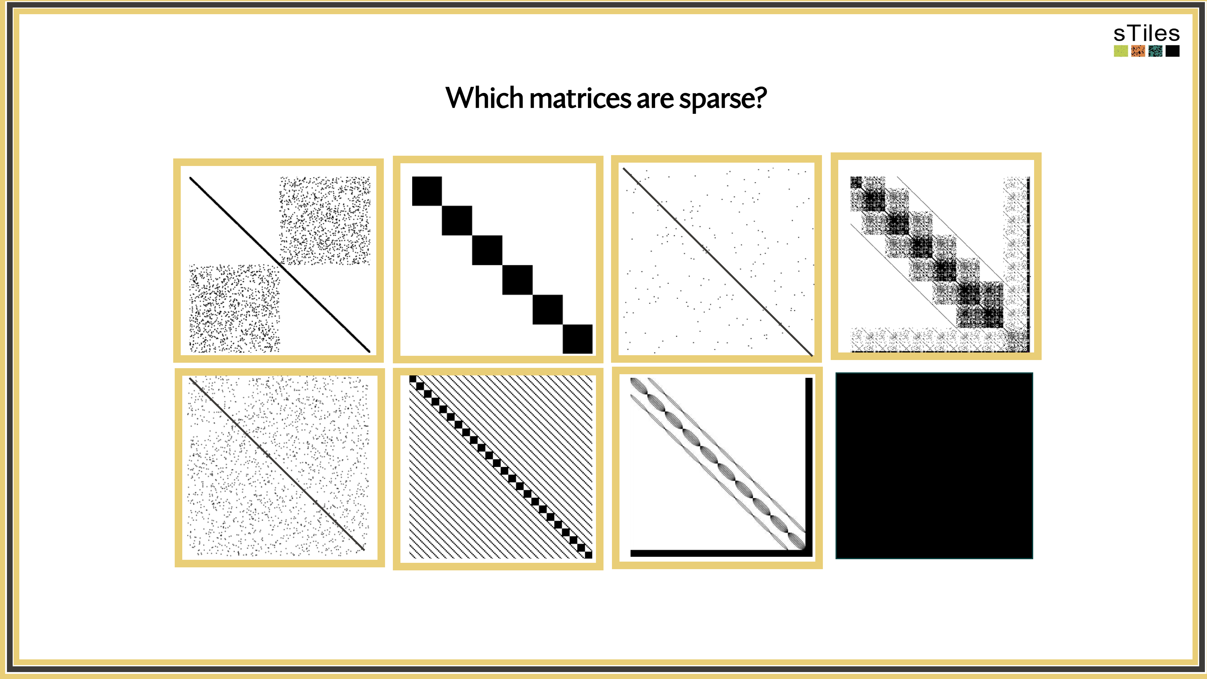
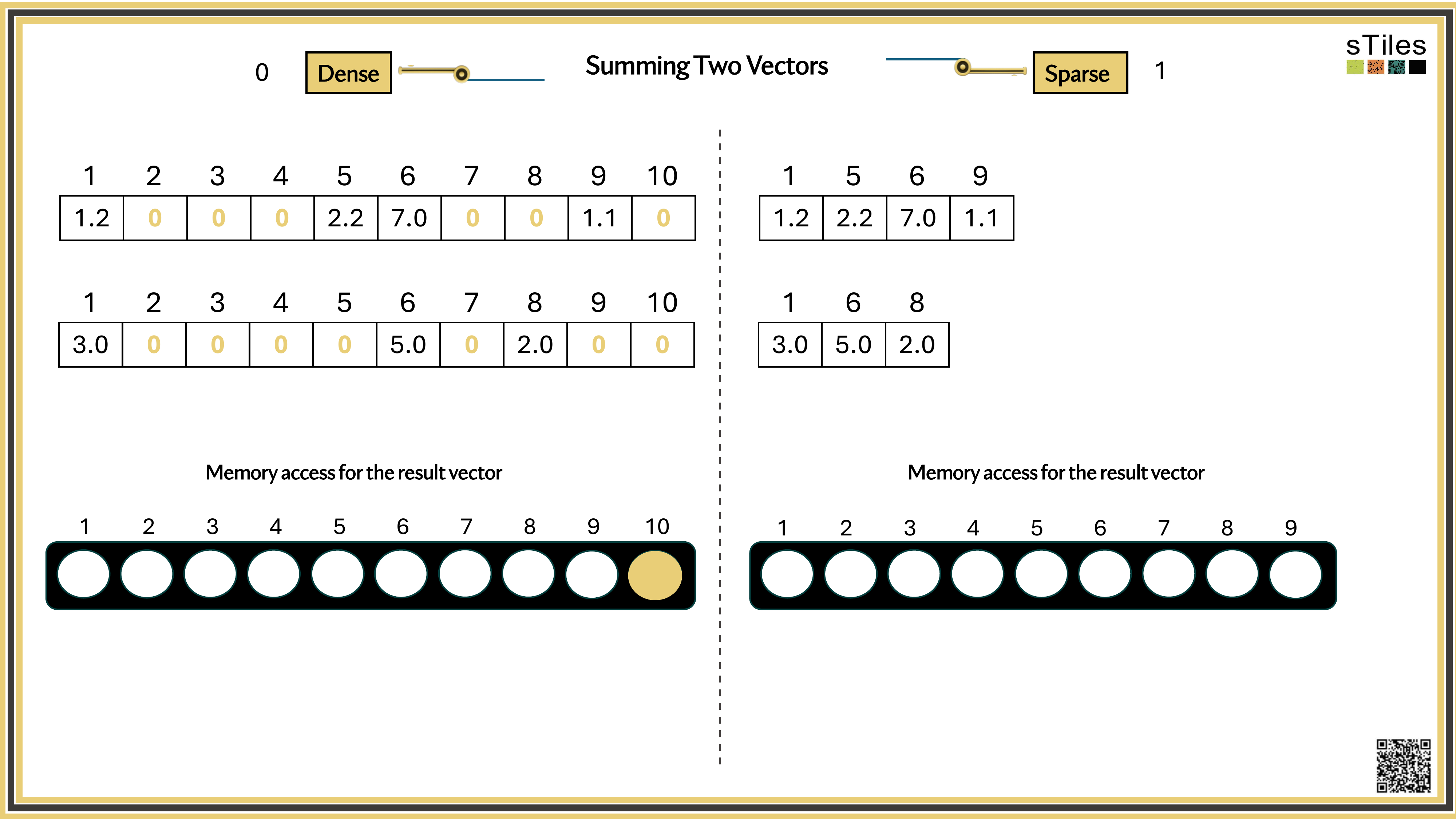
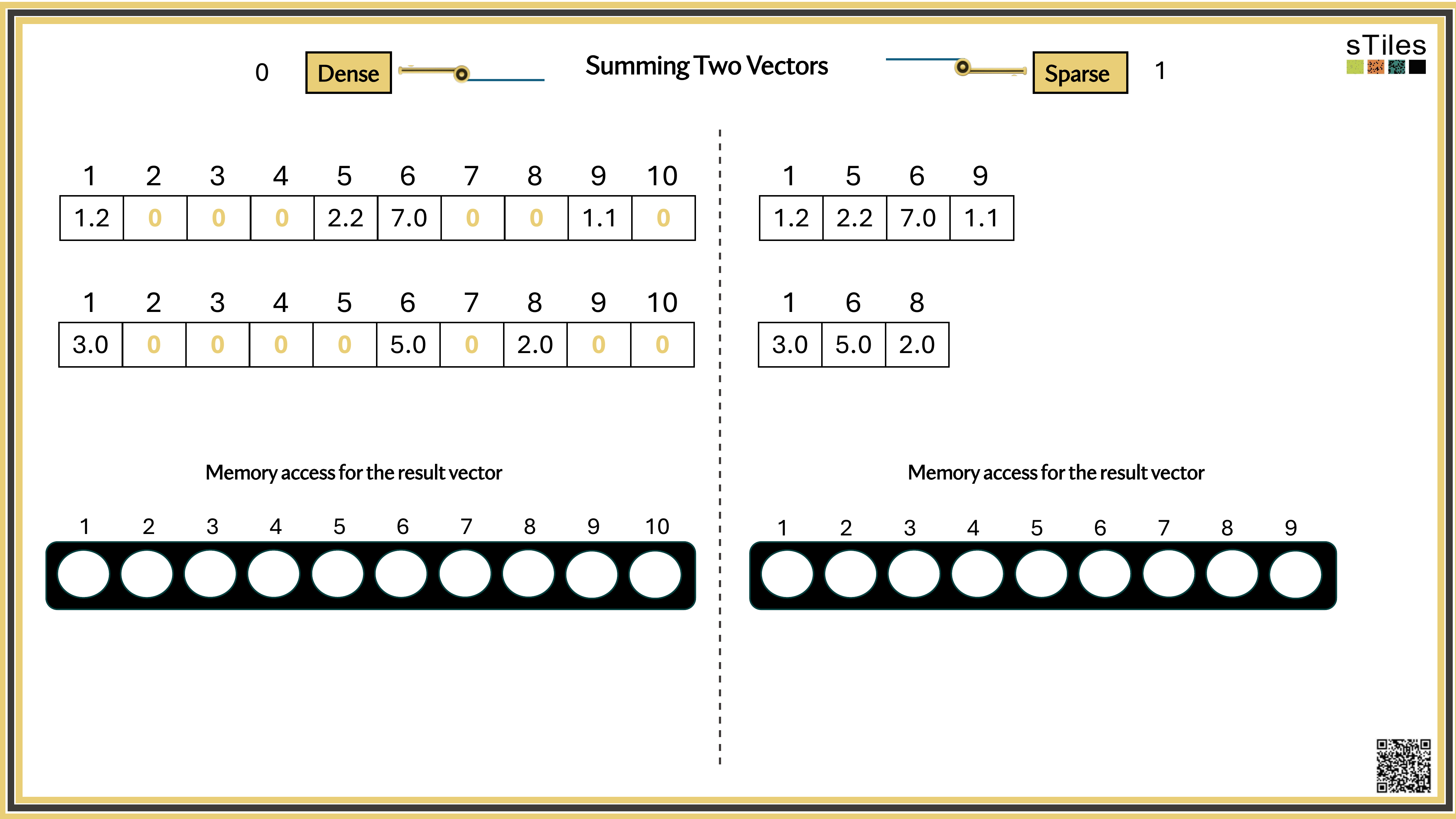
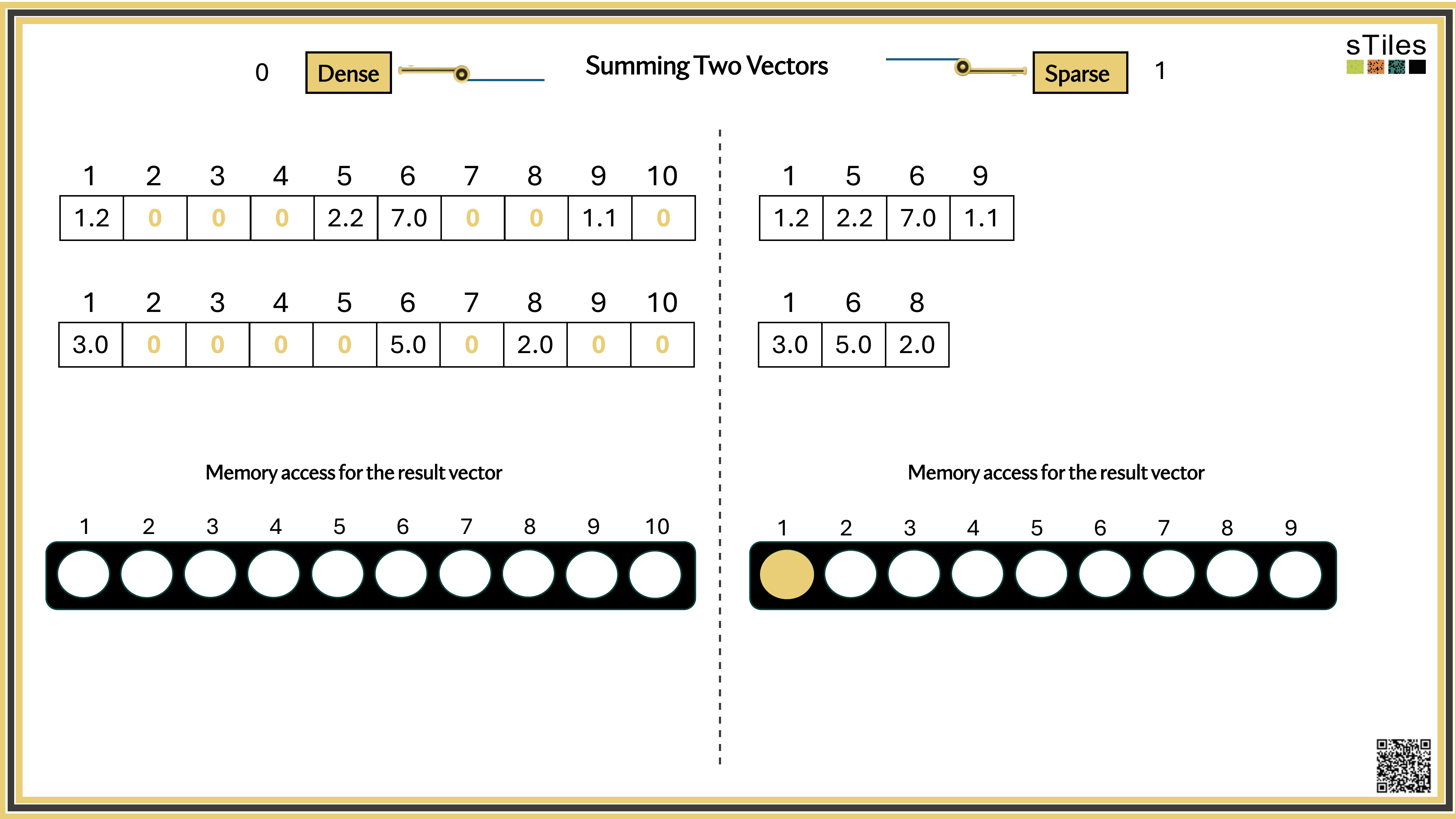
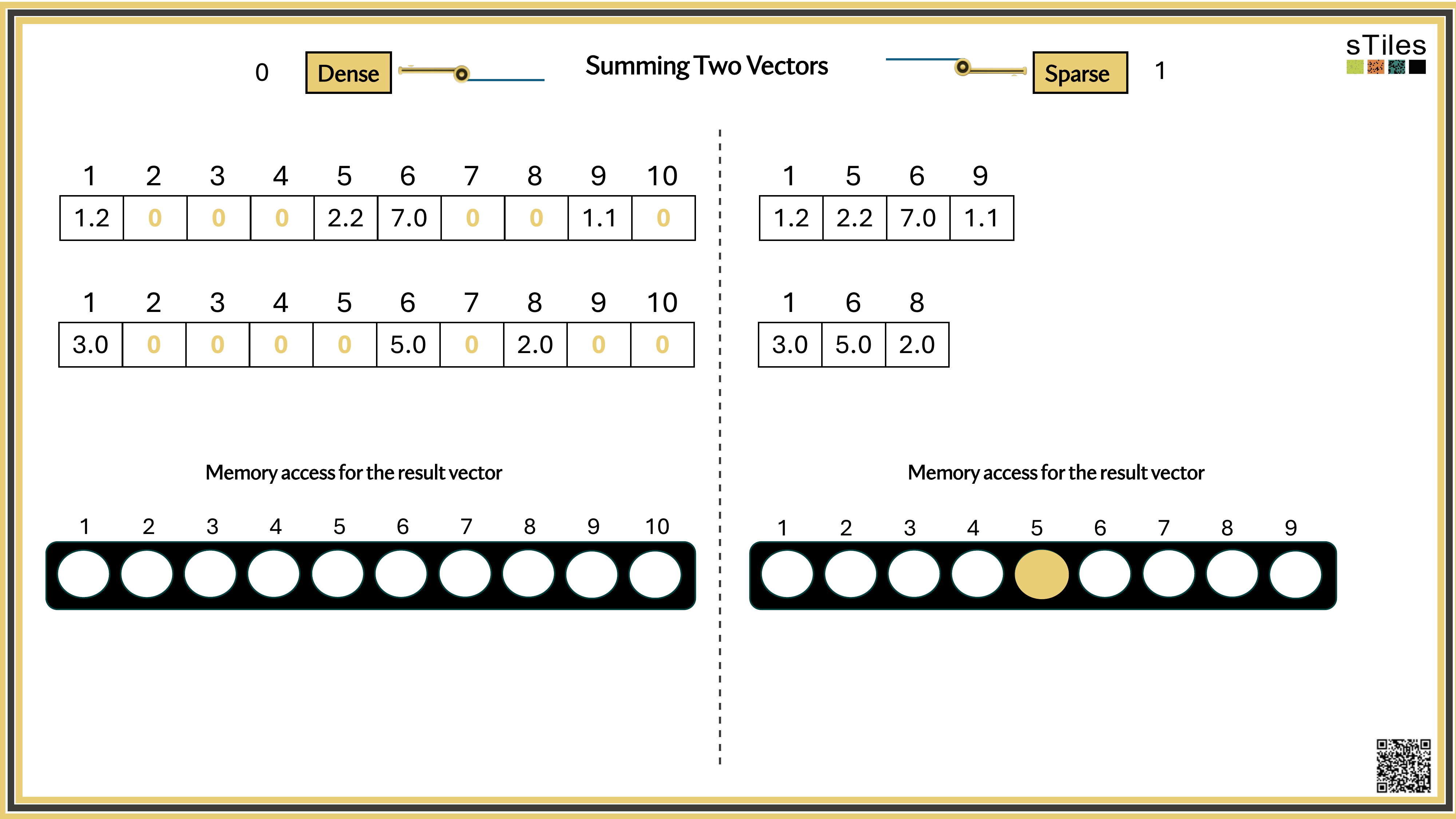
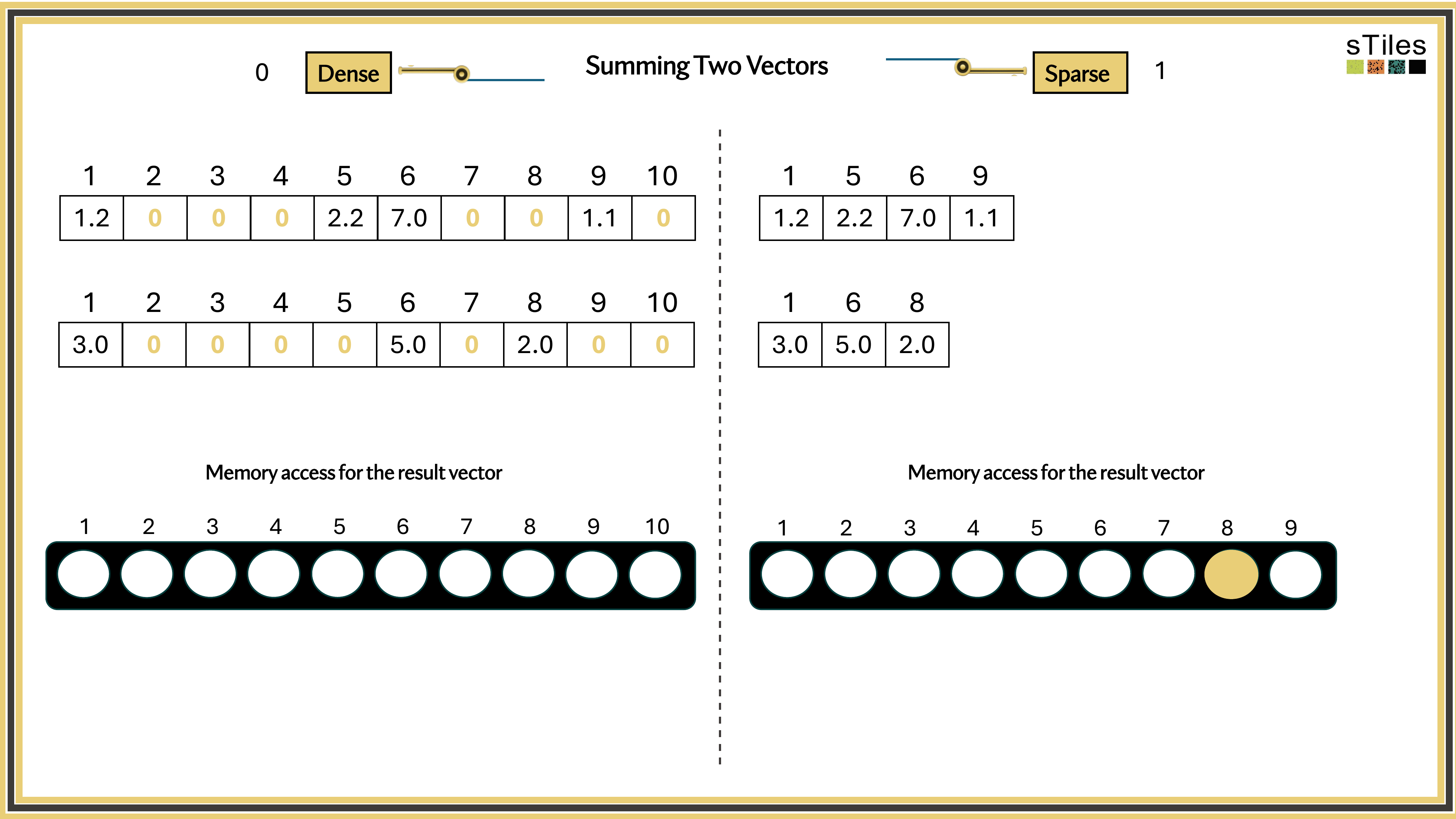
Most entries of A are zero, your model has conditional independence: most parameters don't directly interact. That gives us a choice.
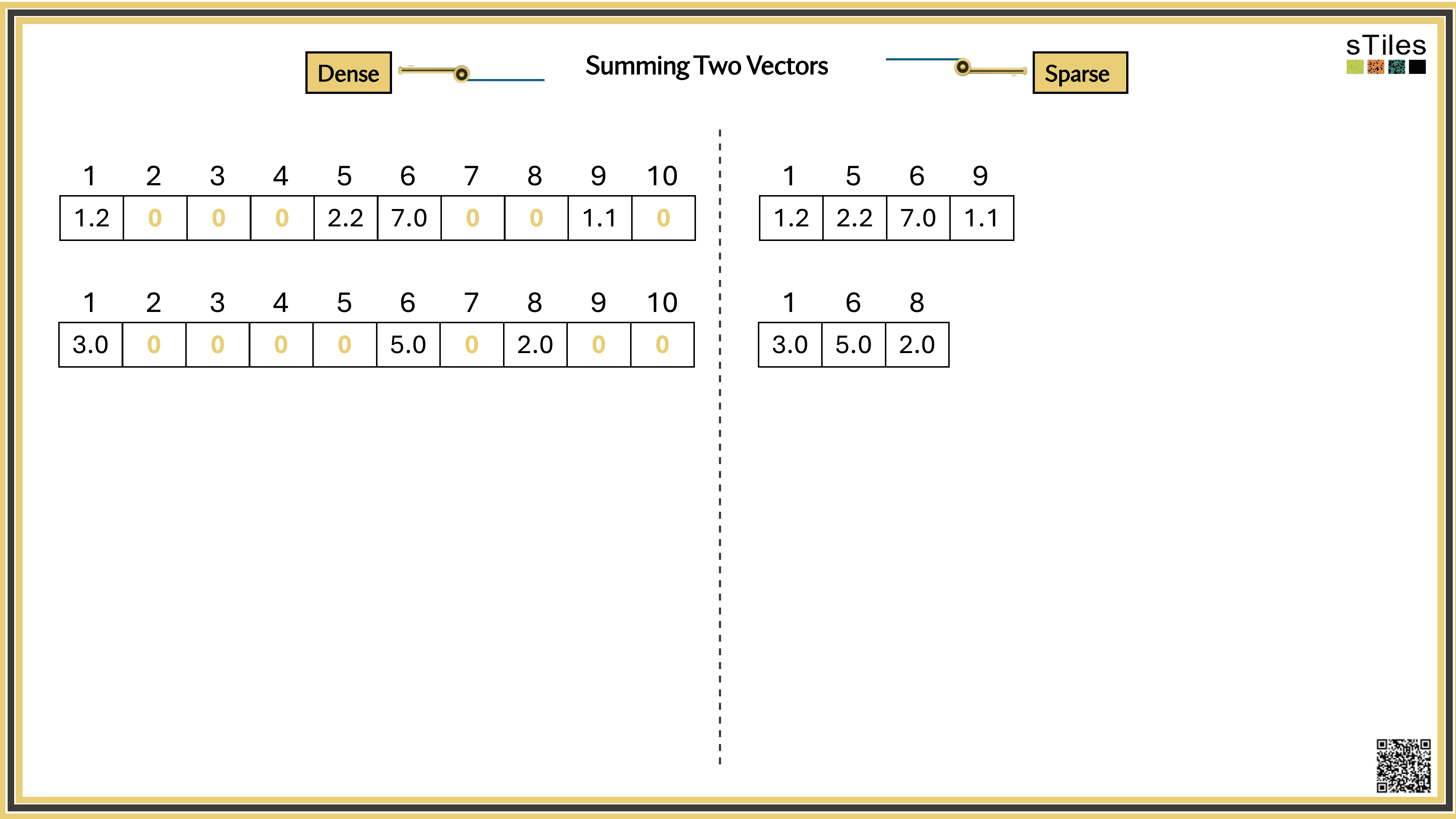
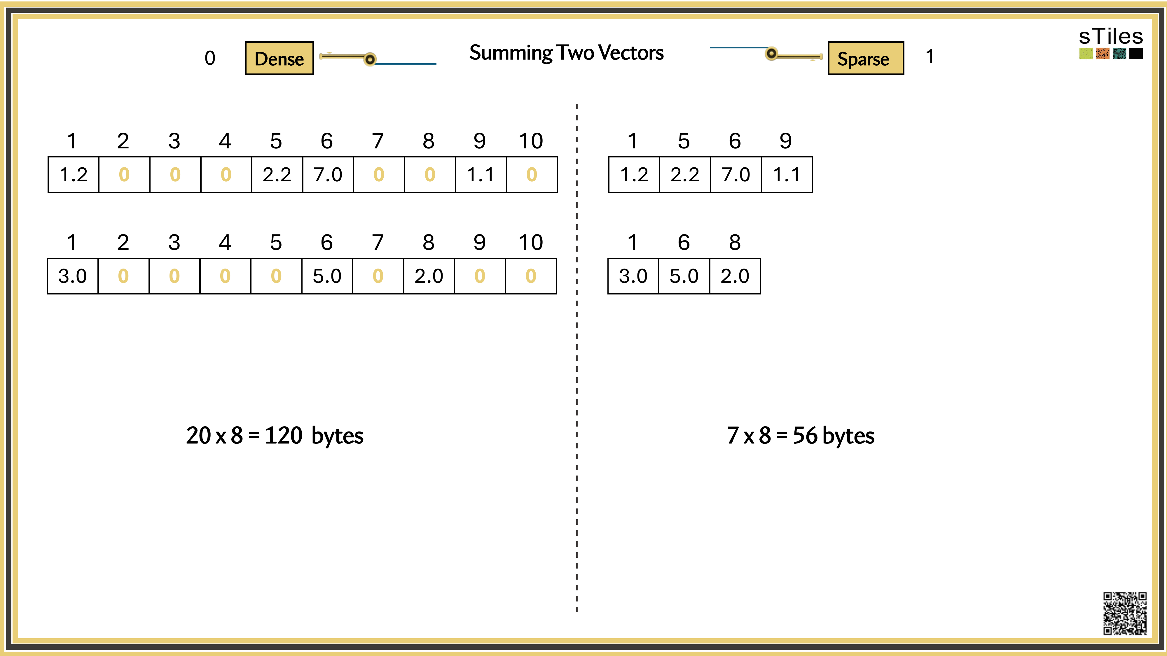
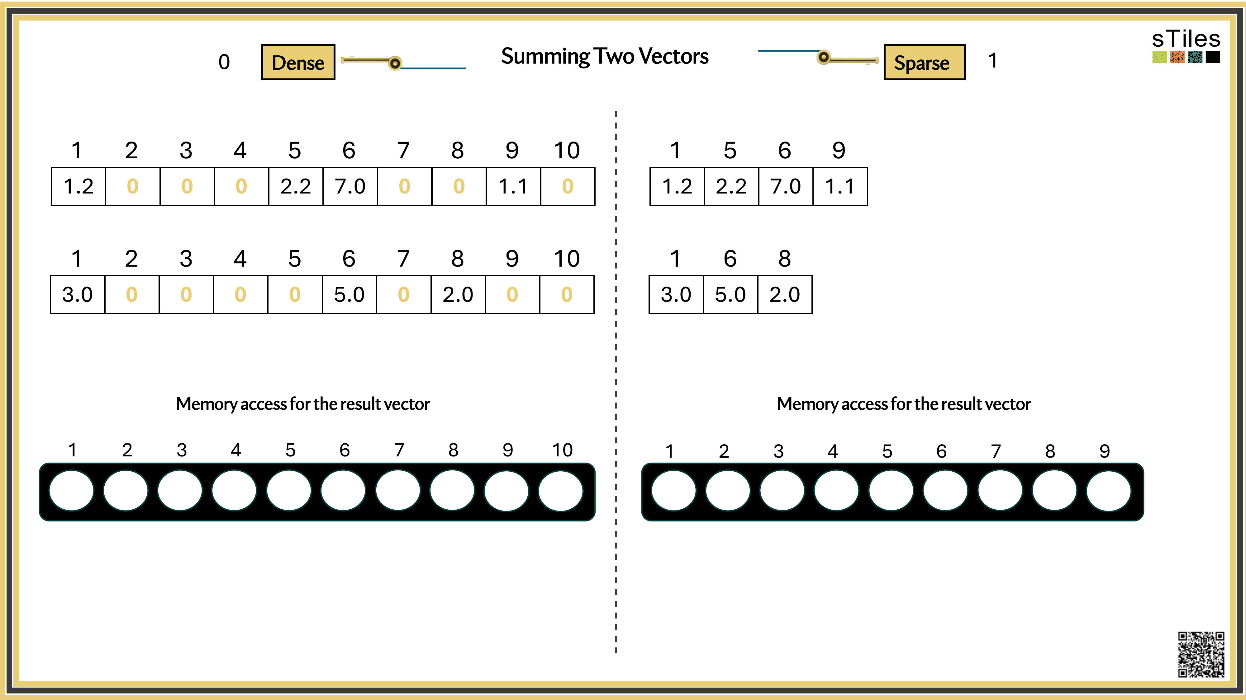
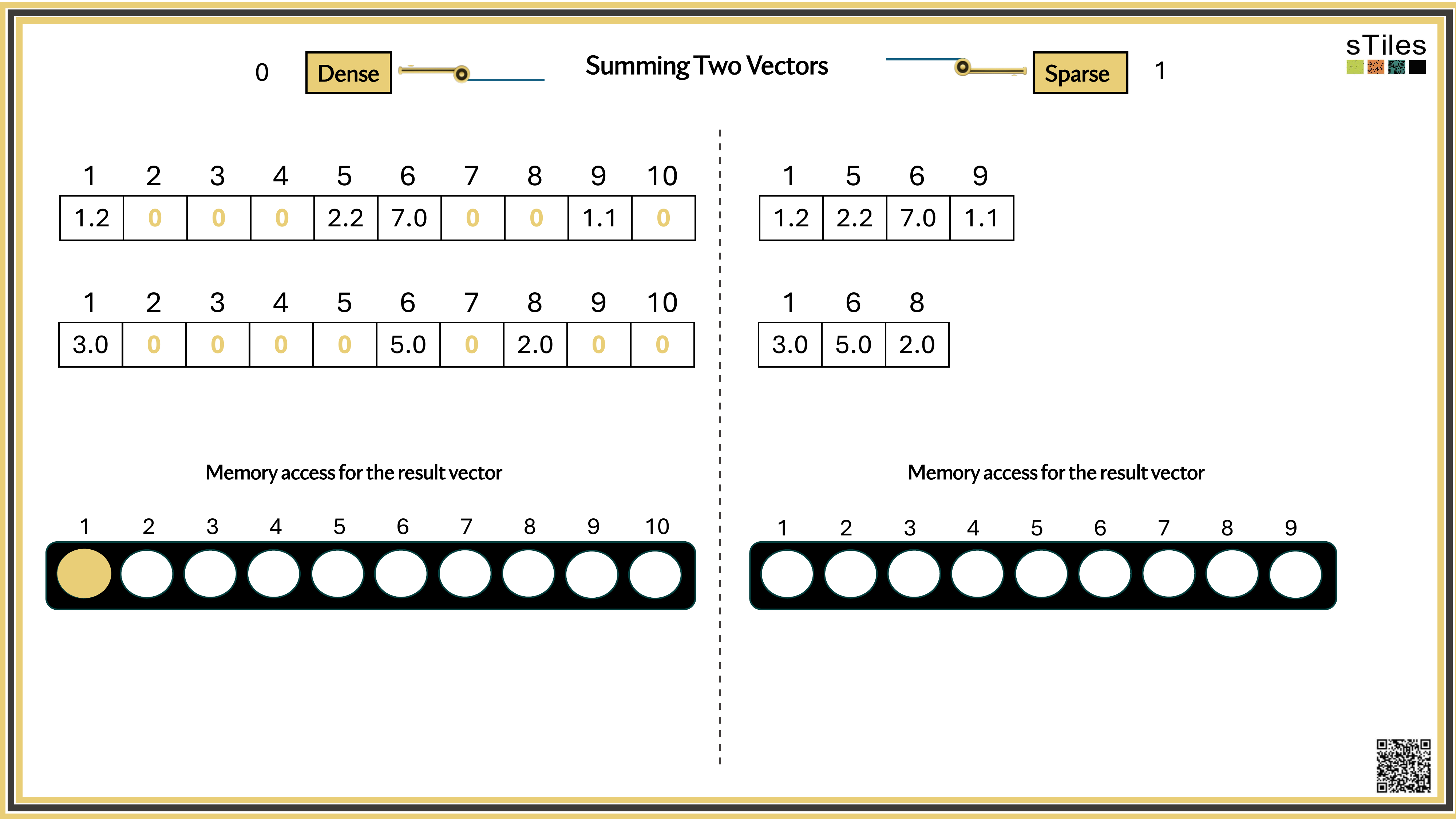
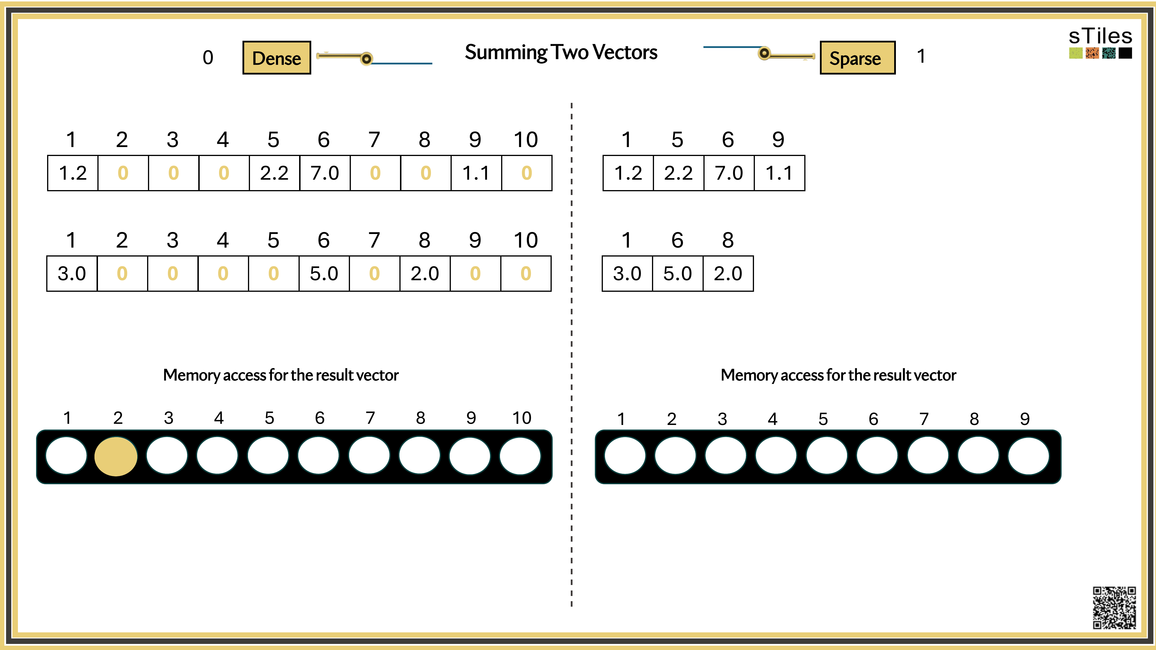
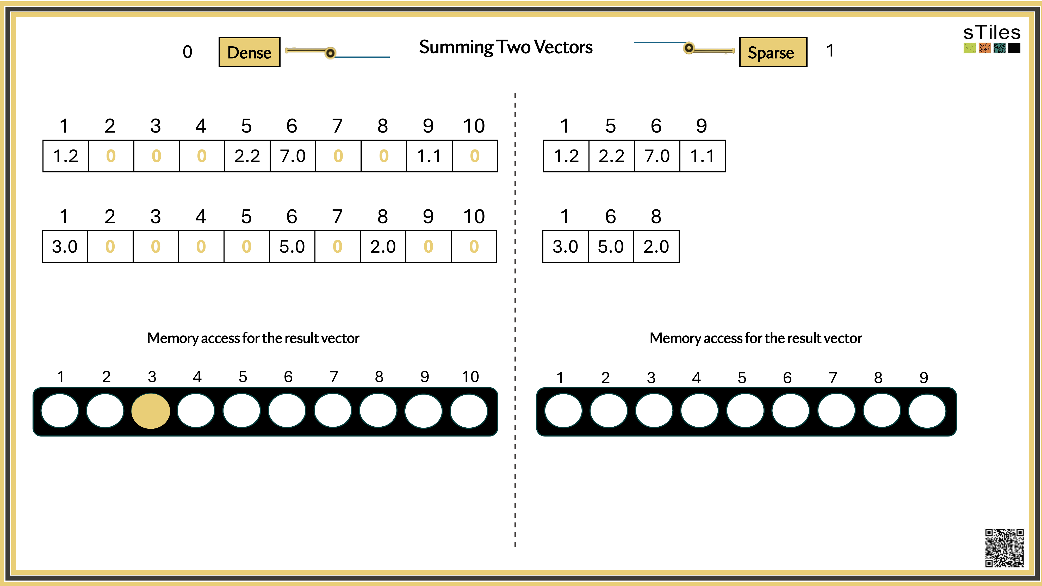
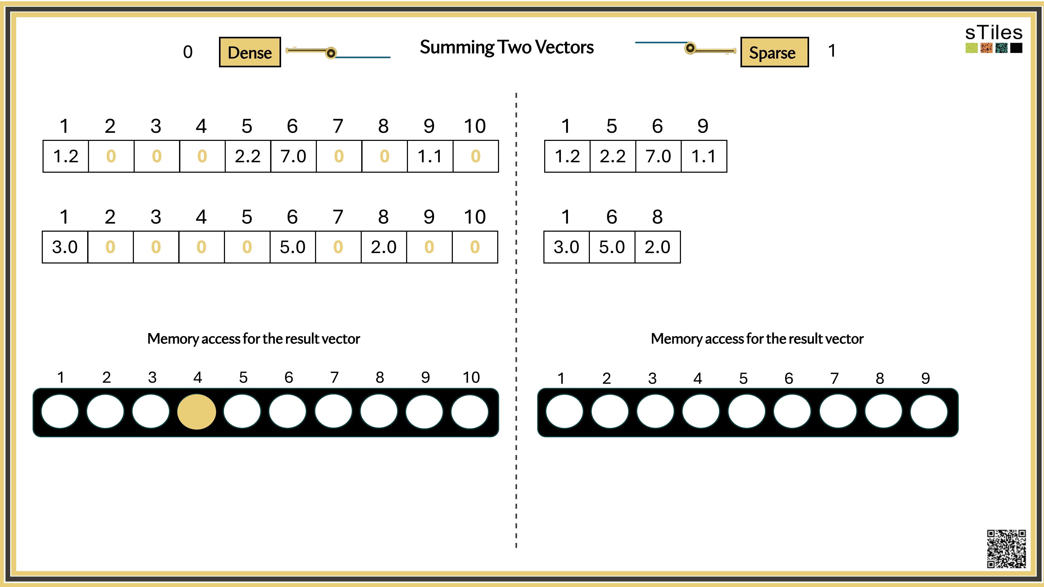
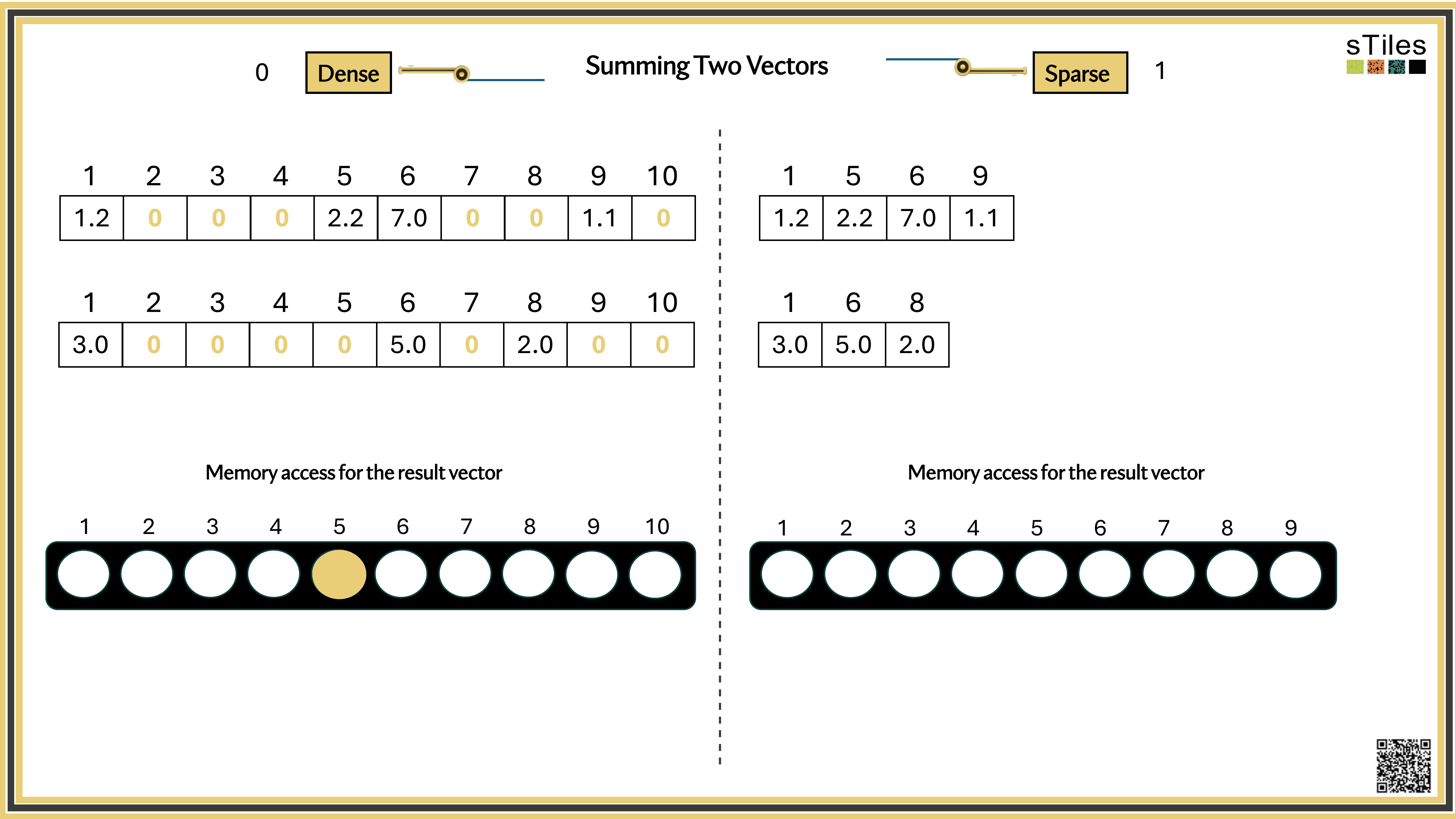
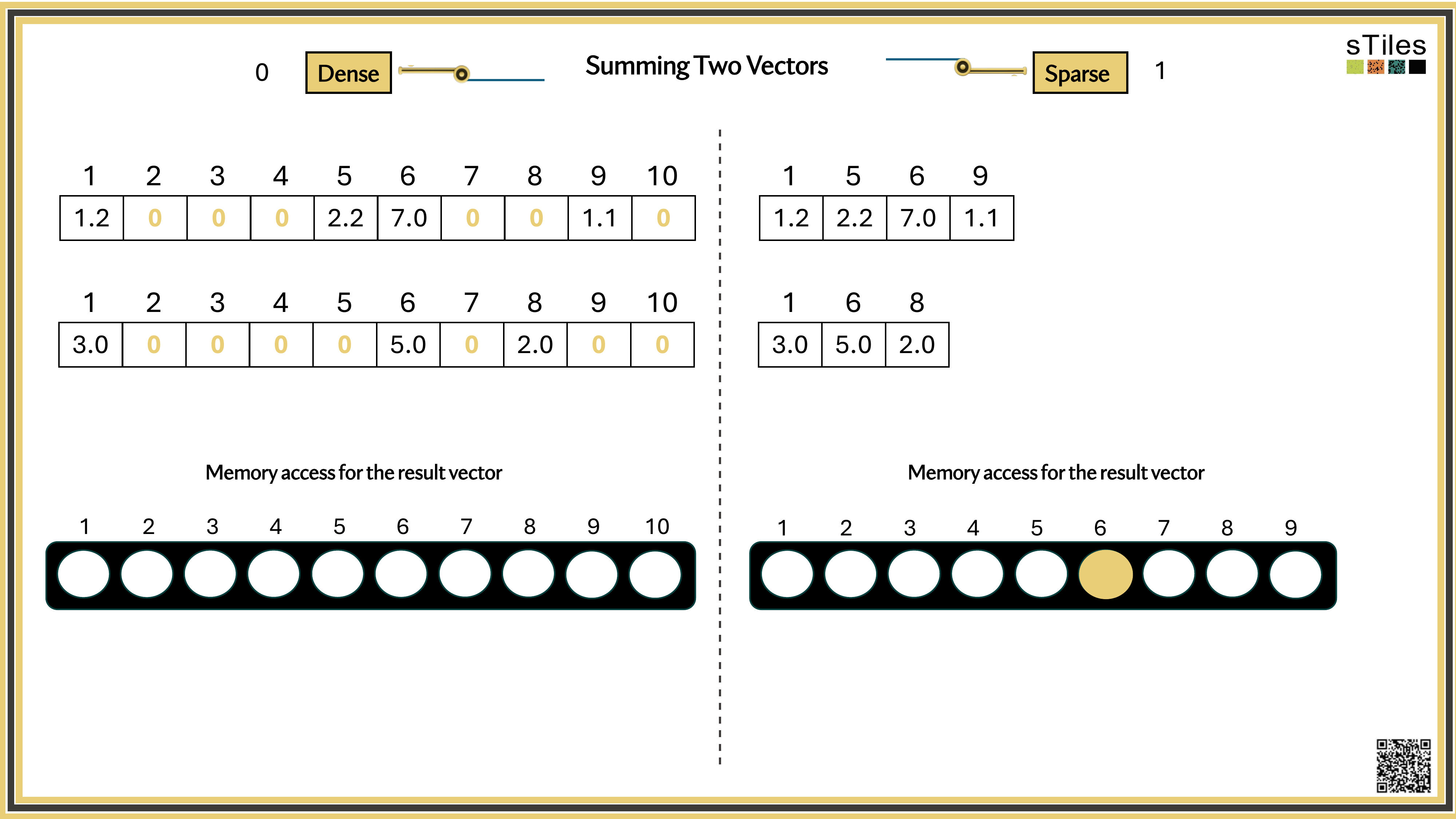
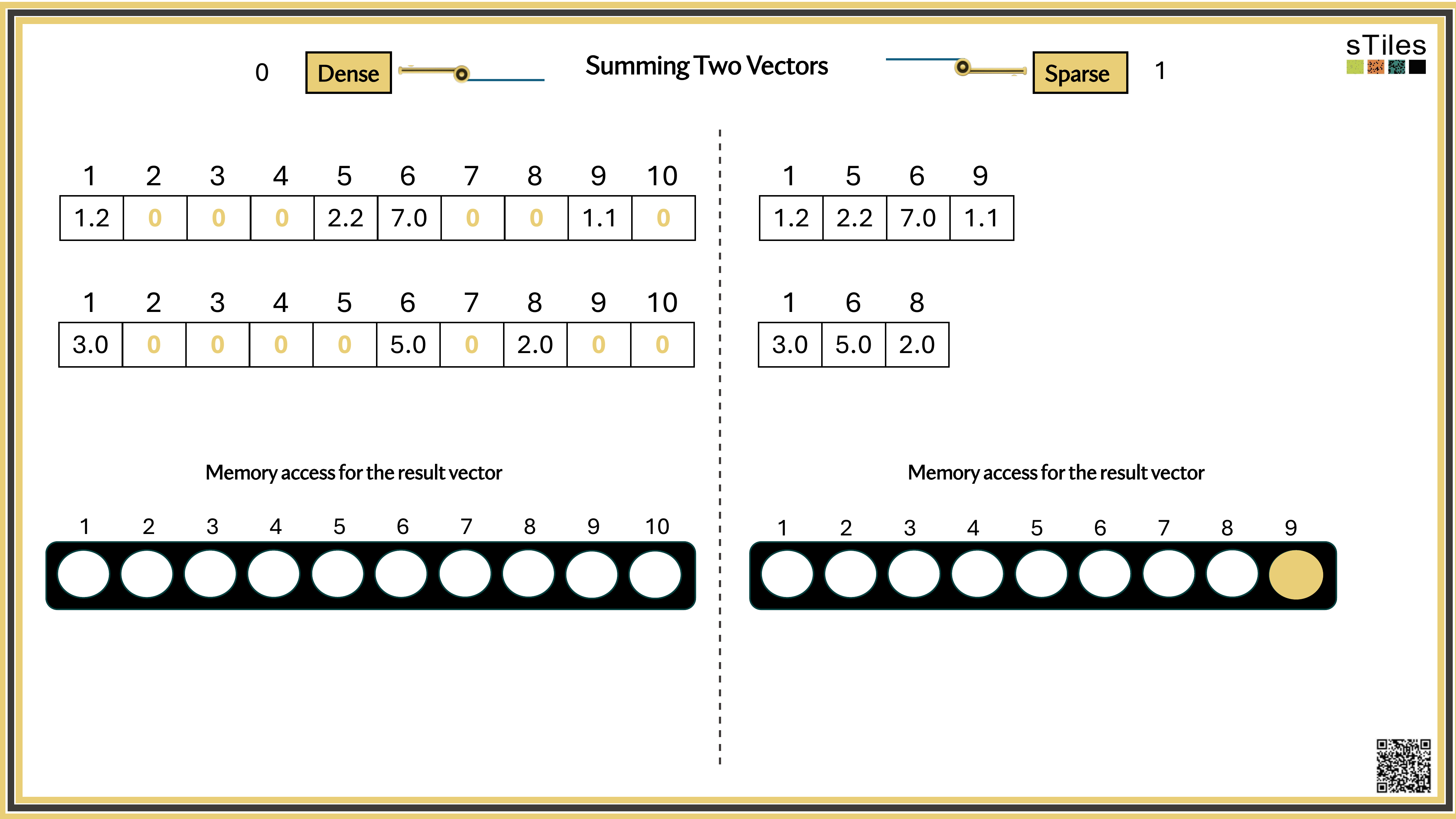
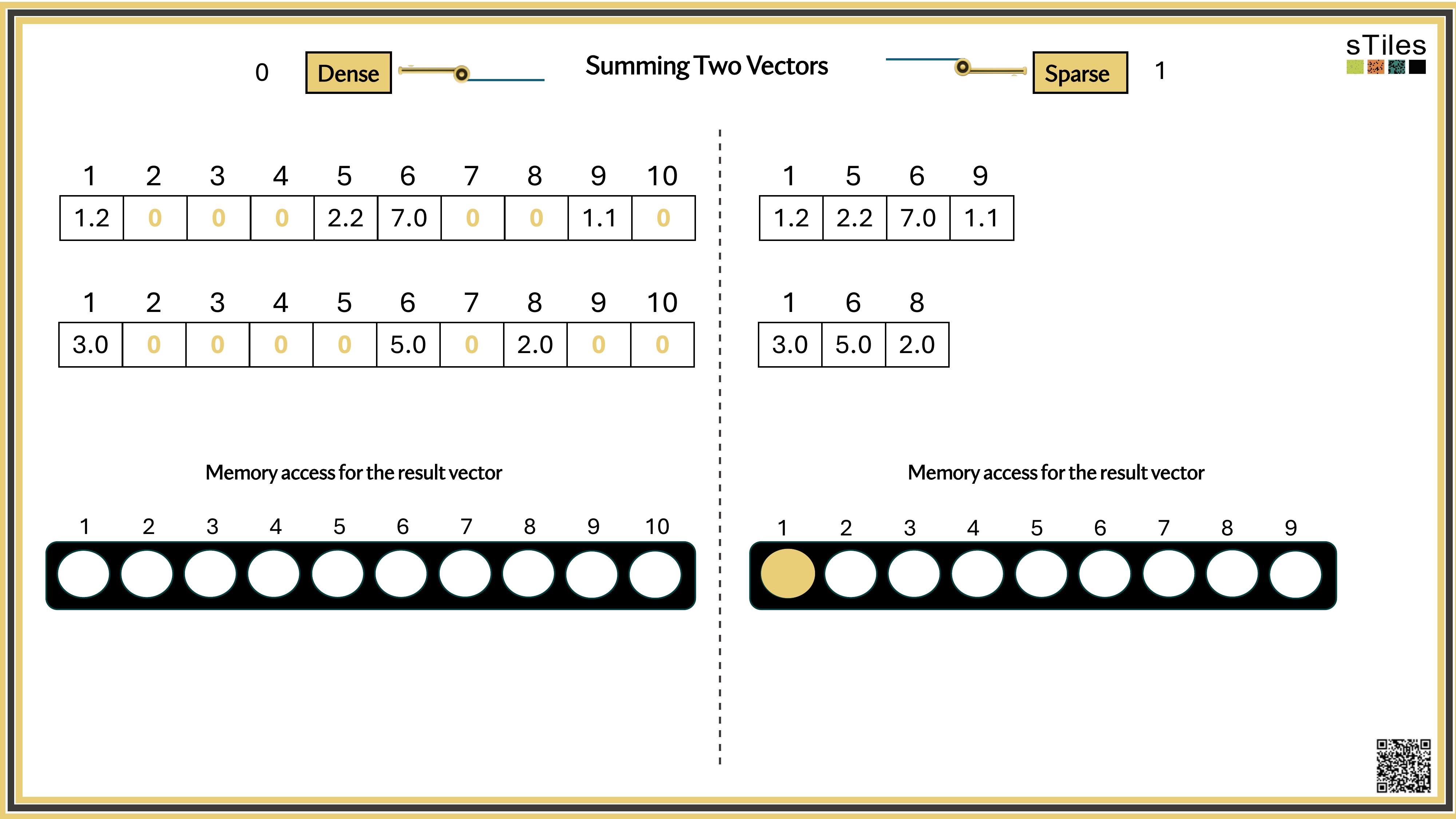
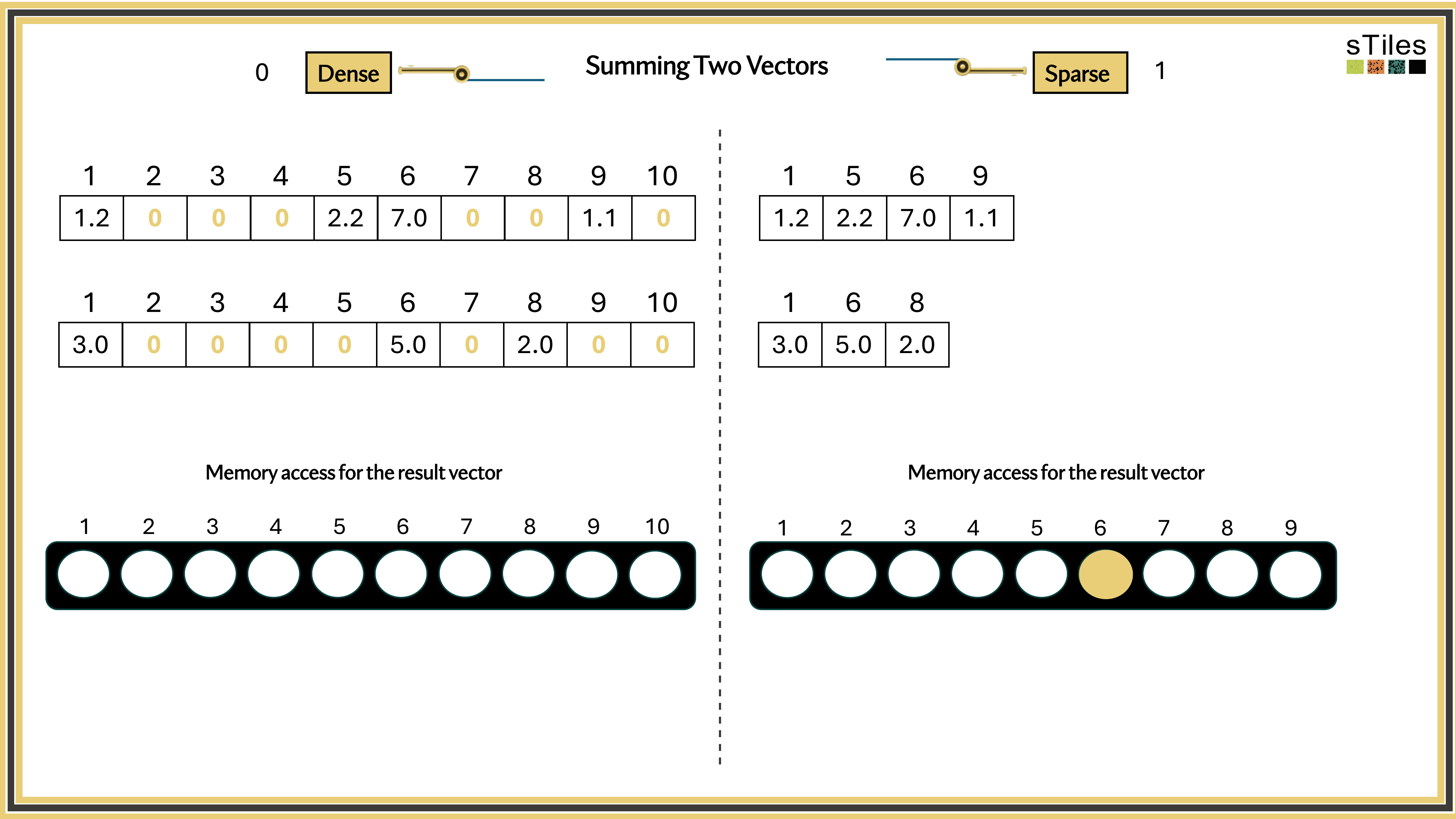
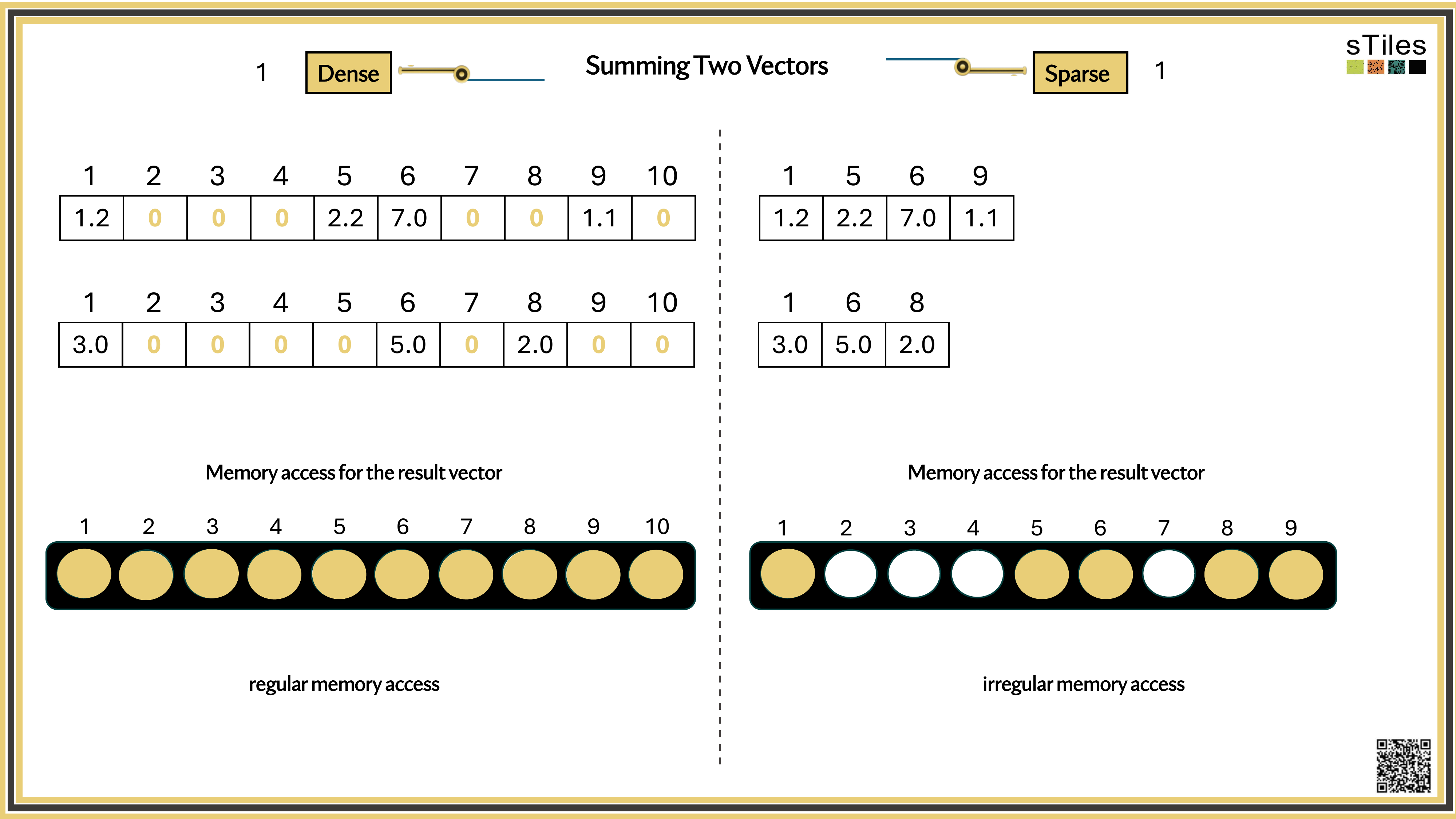
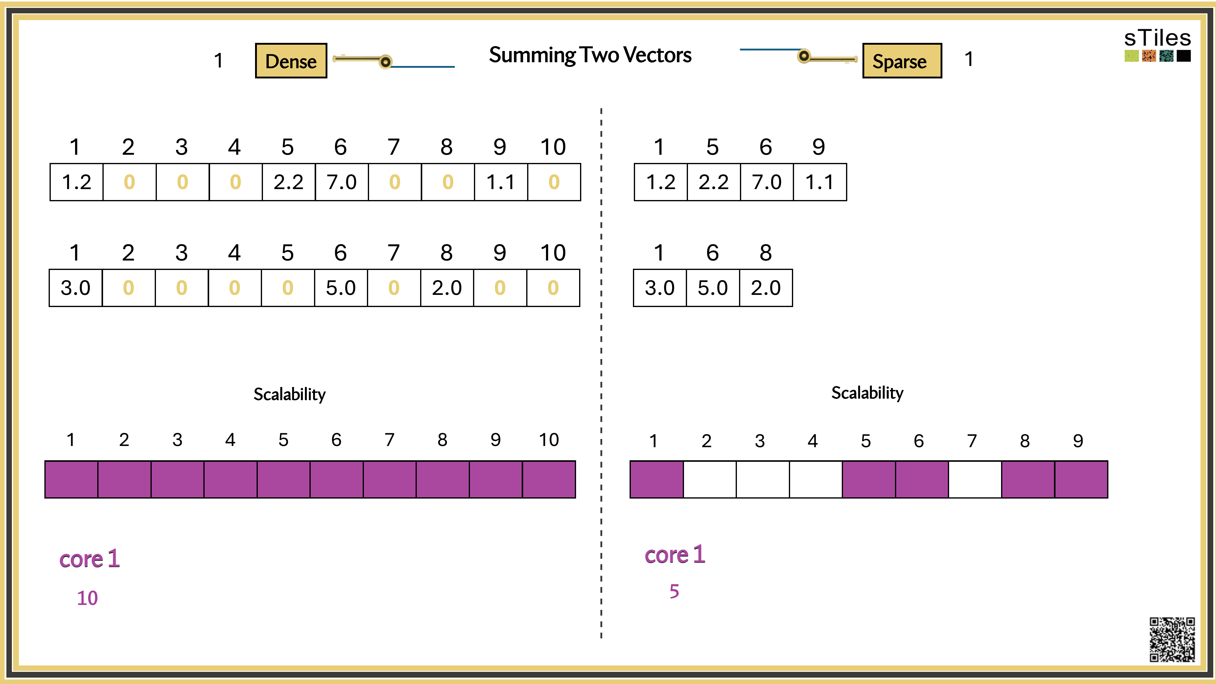
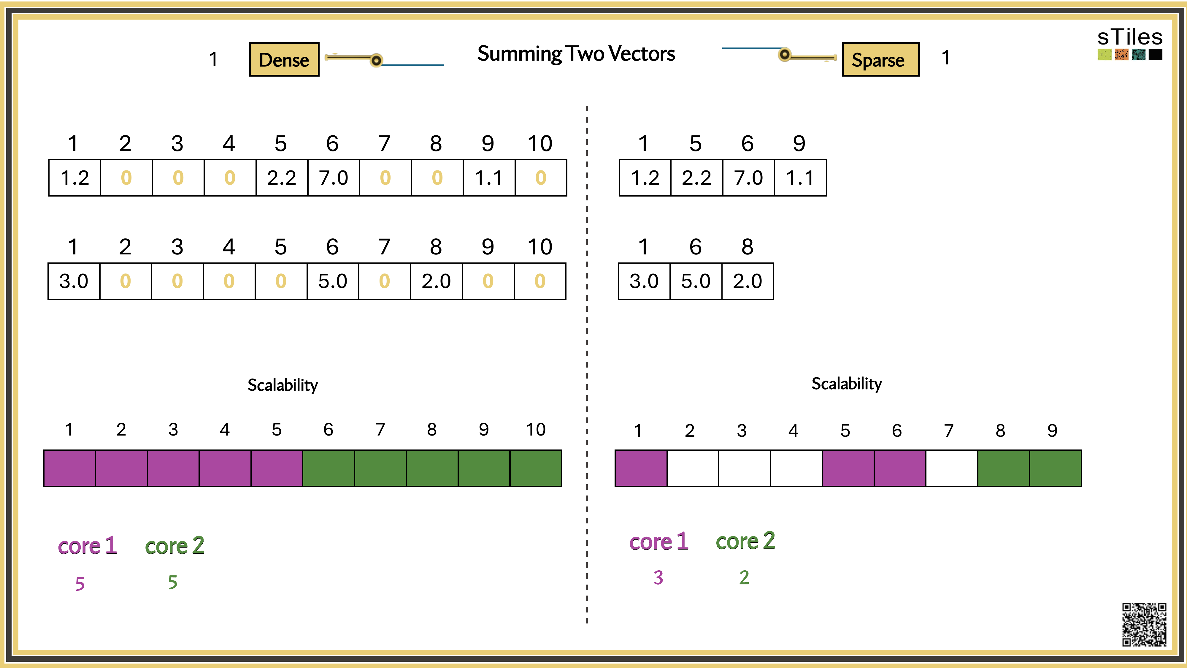
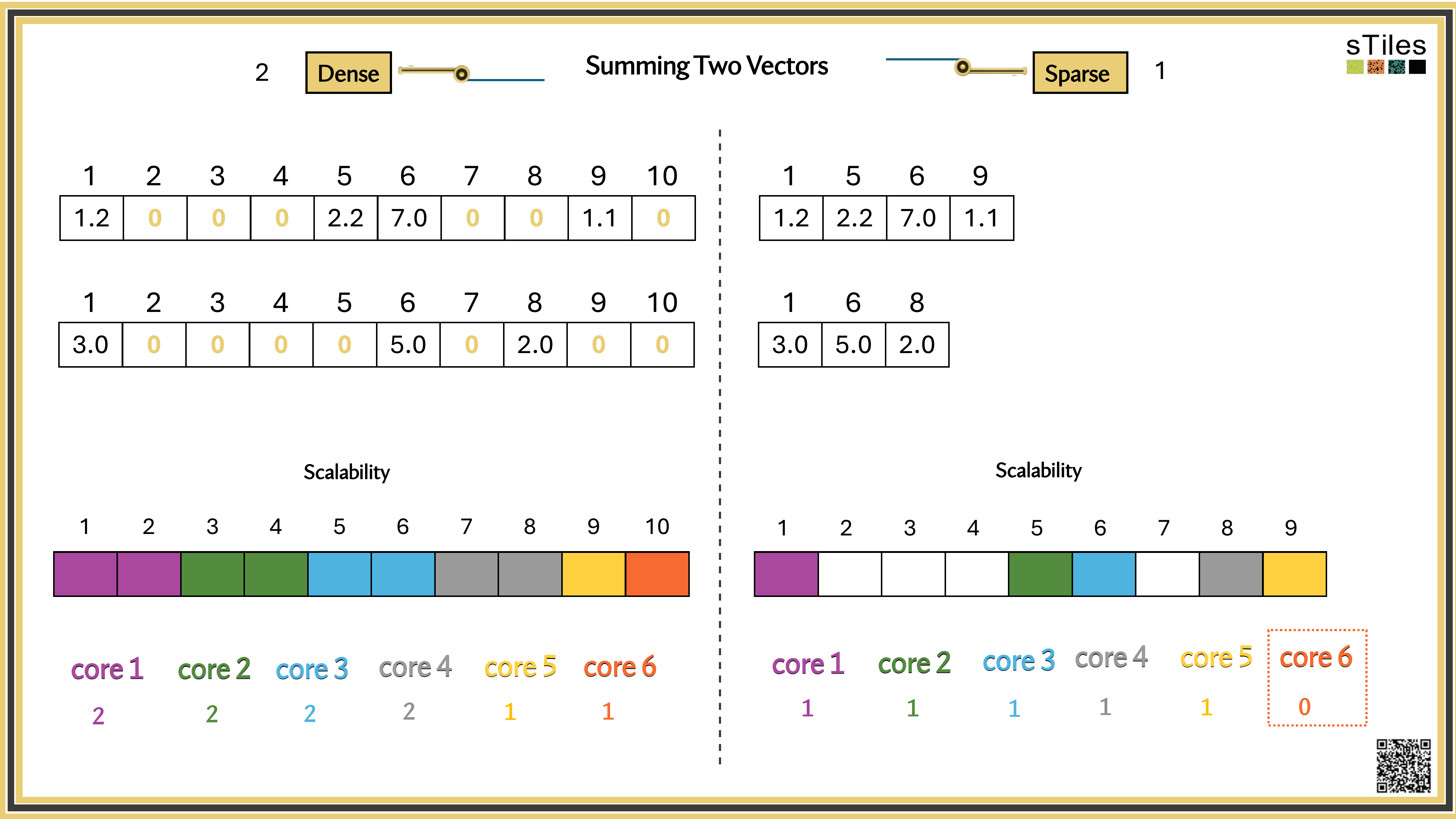
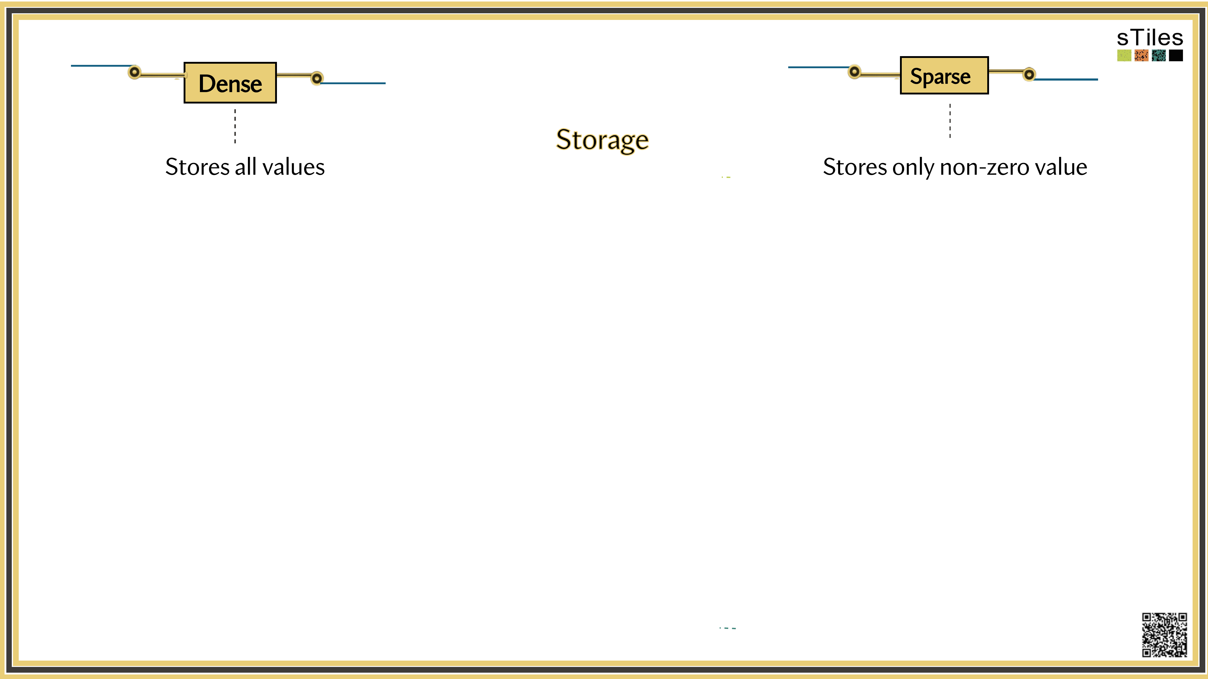
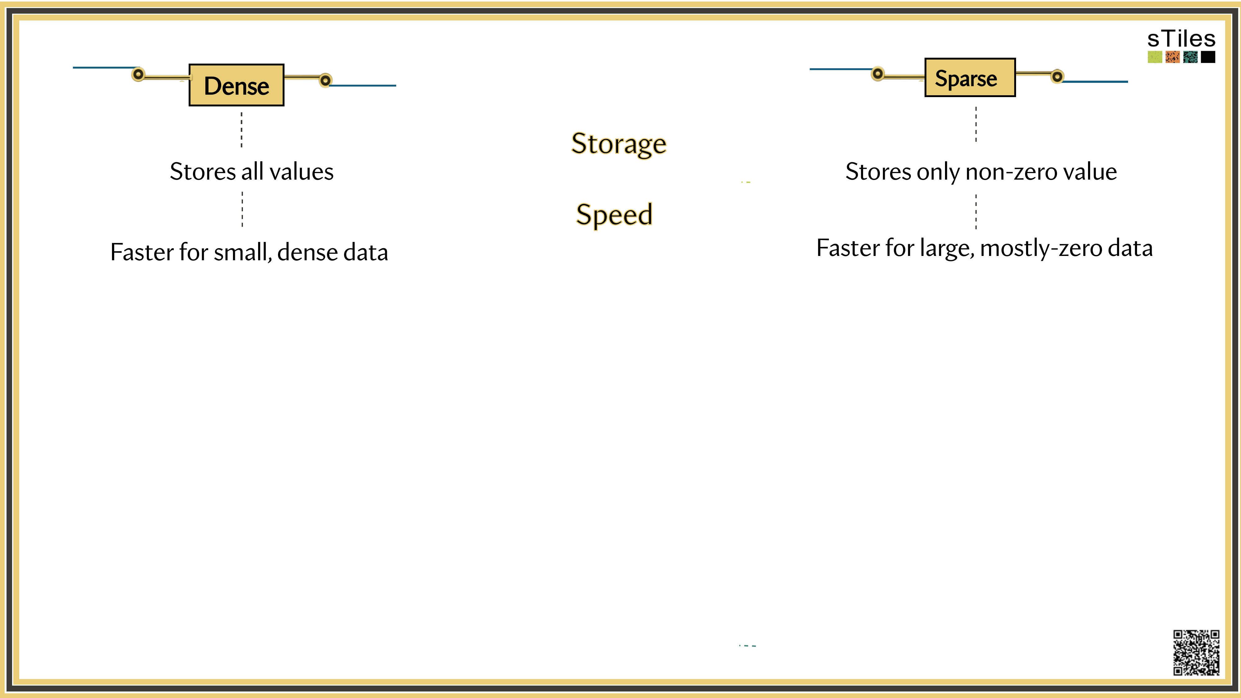
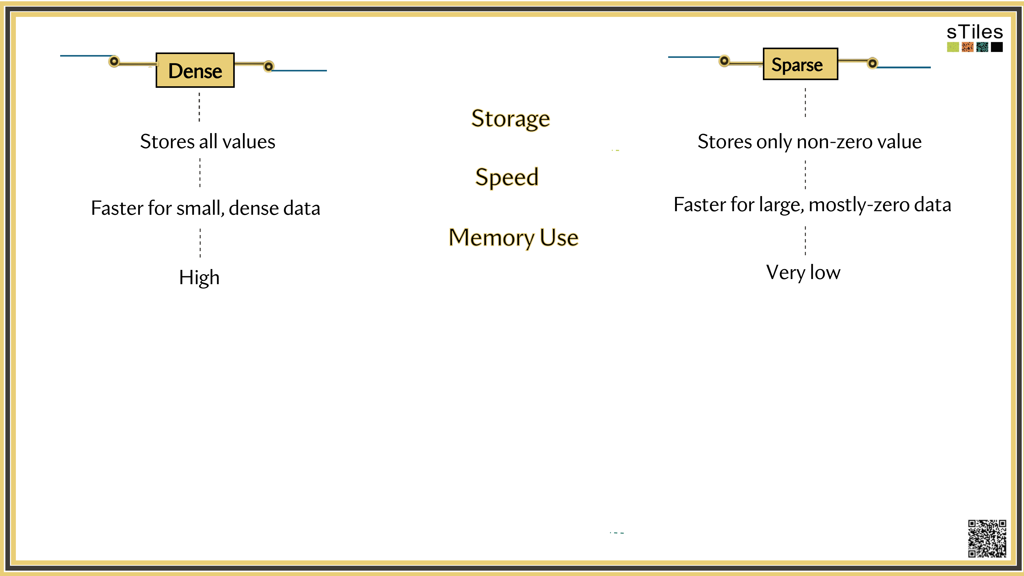
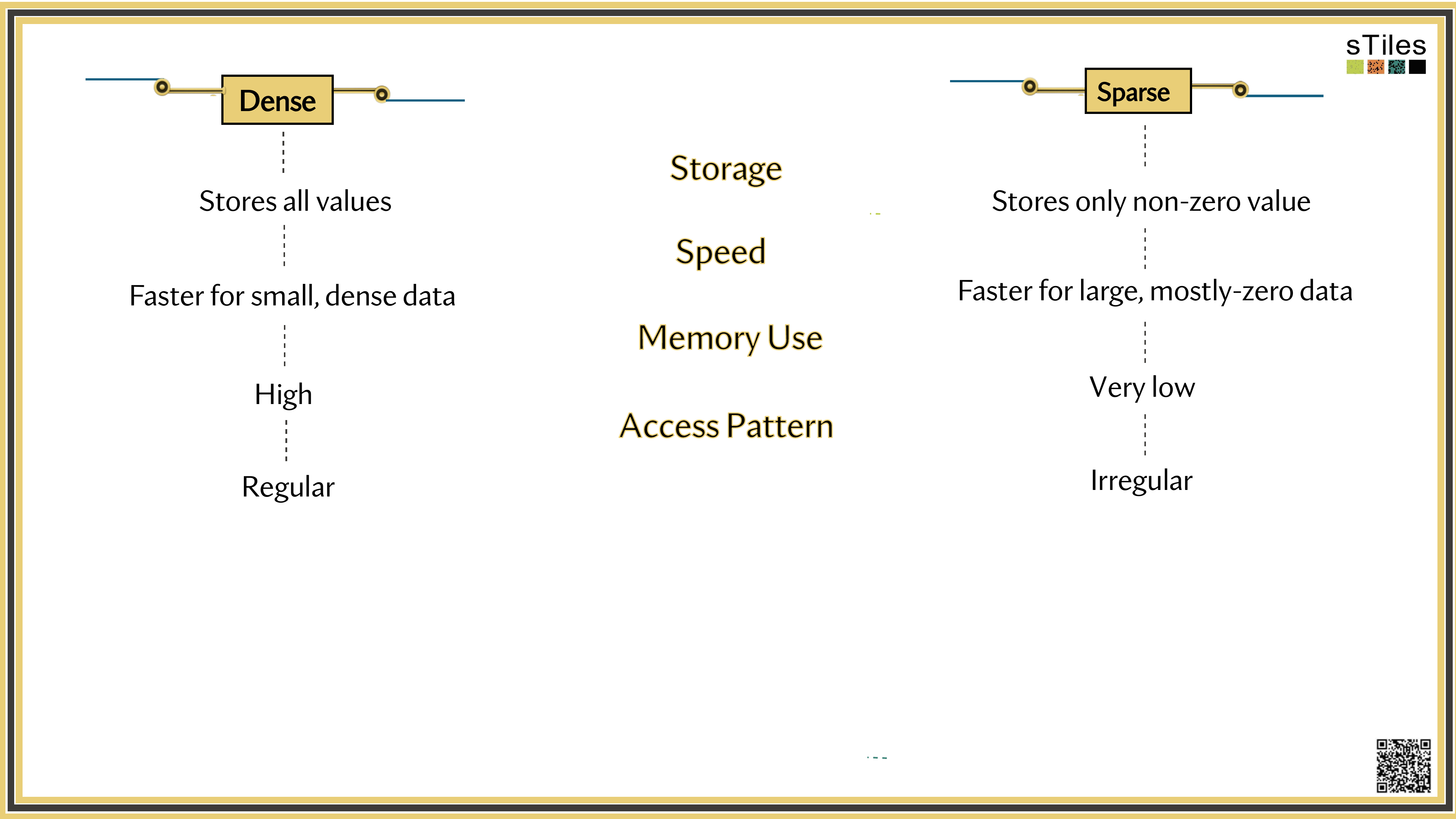
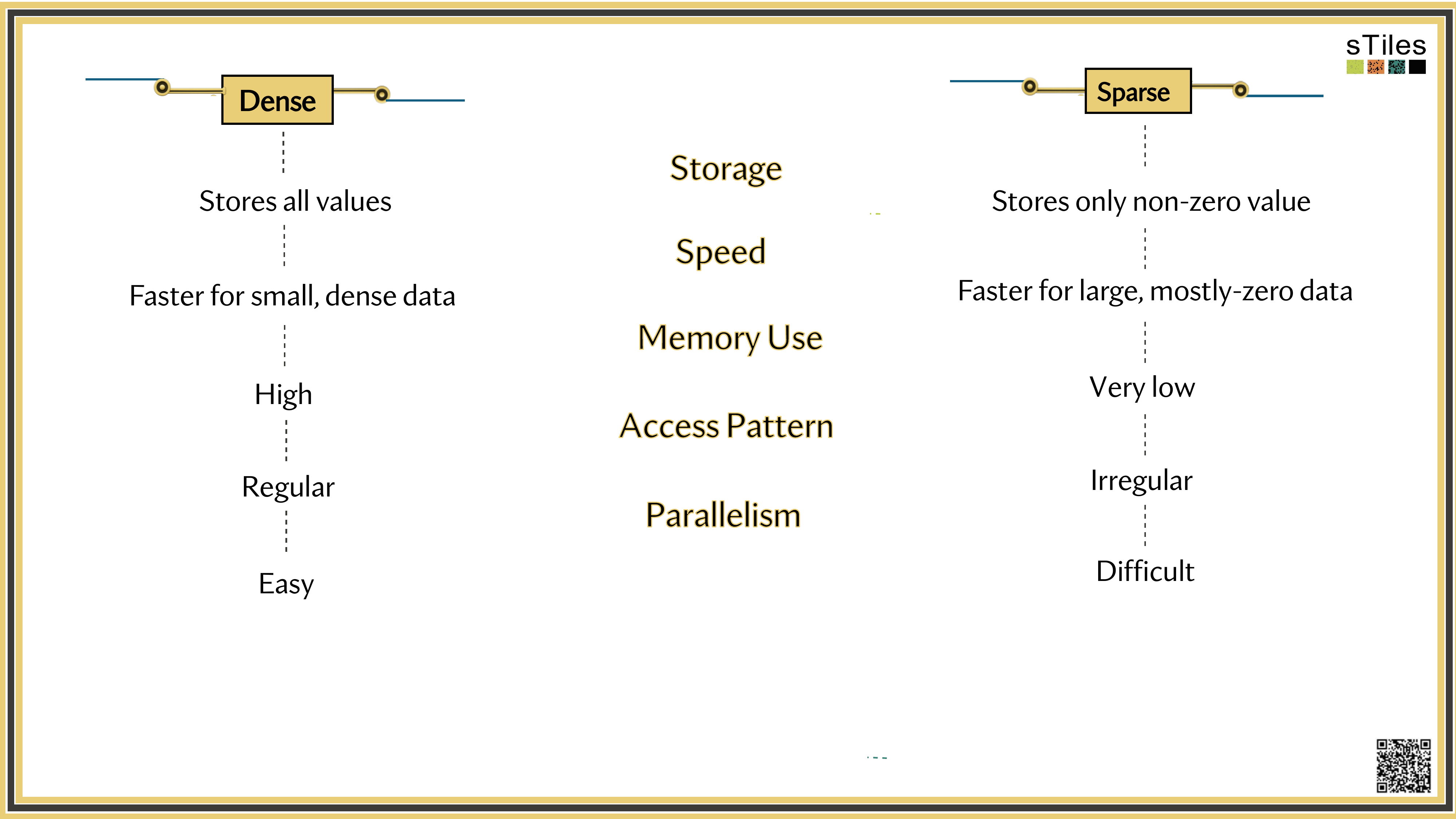
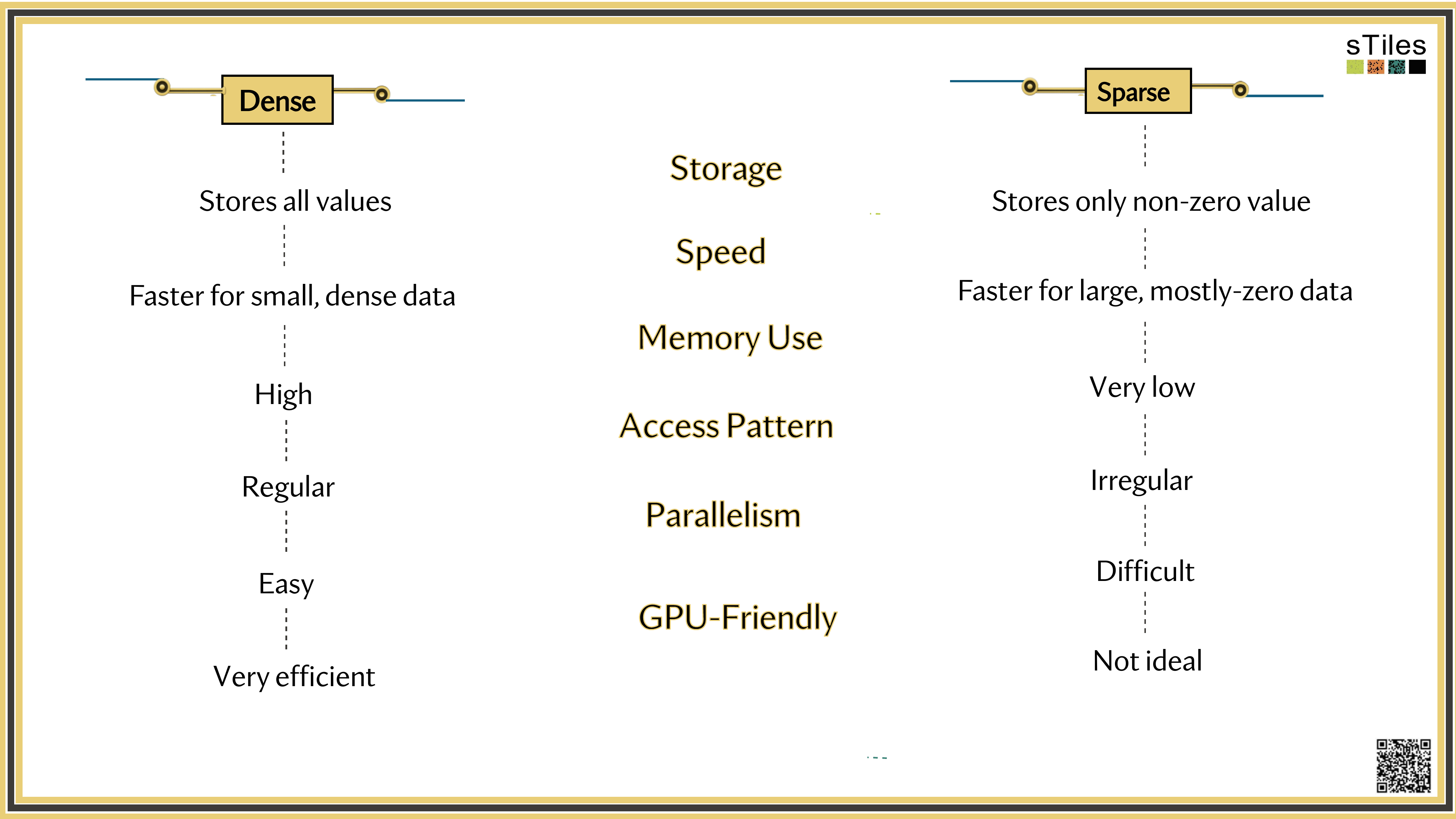
Dense solver
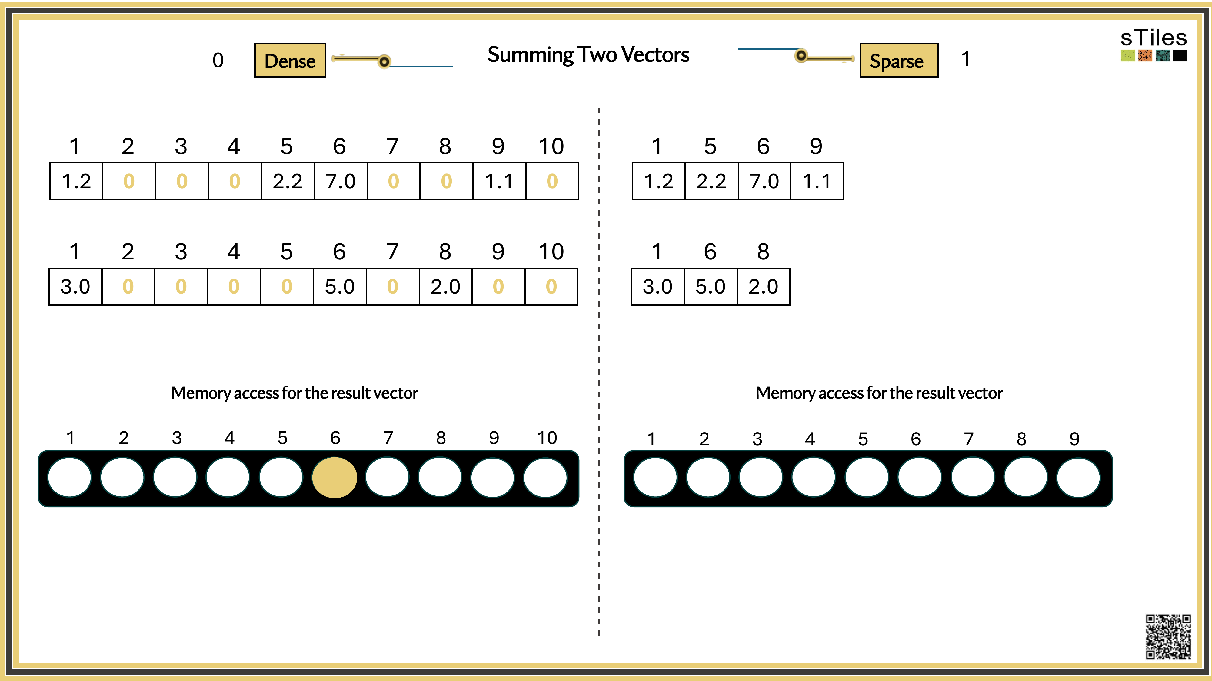
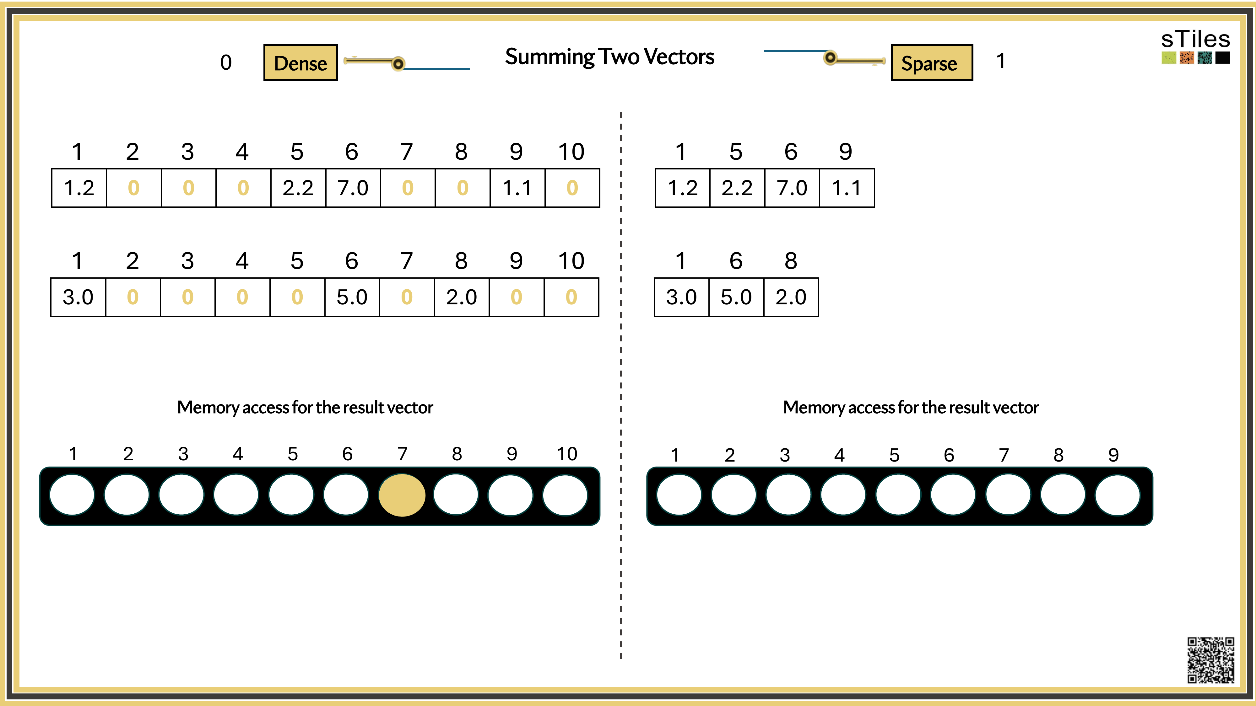
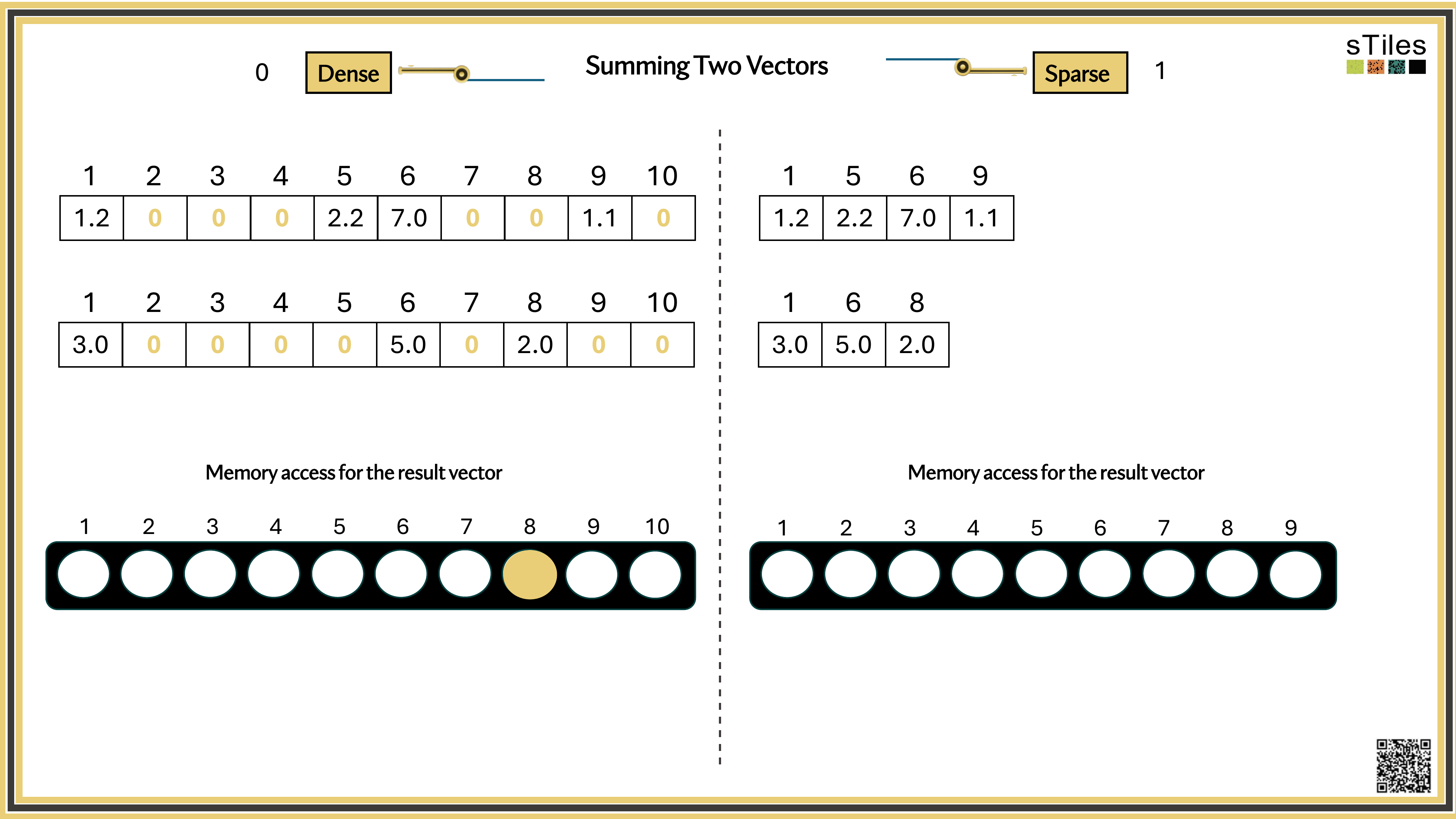
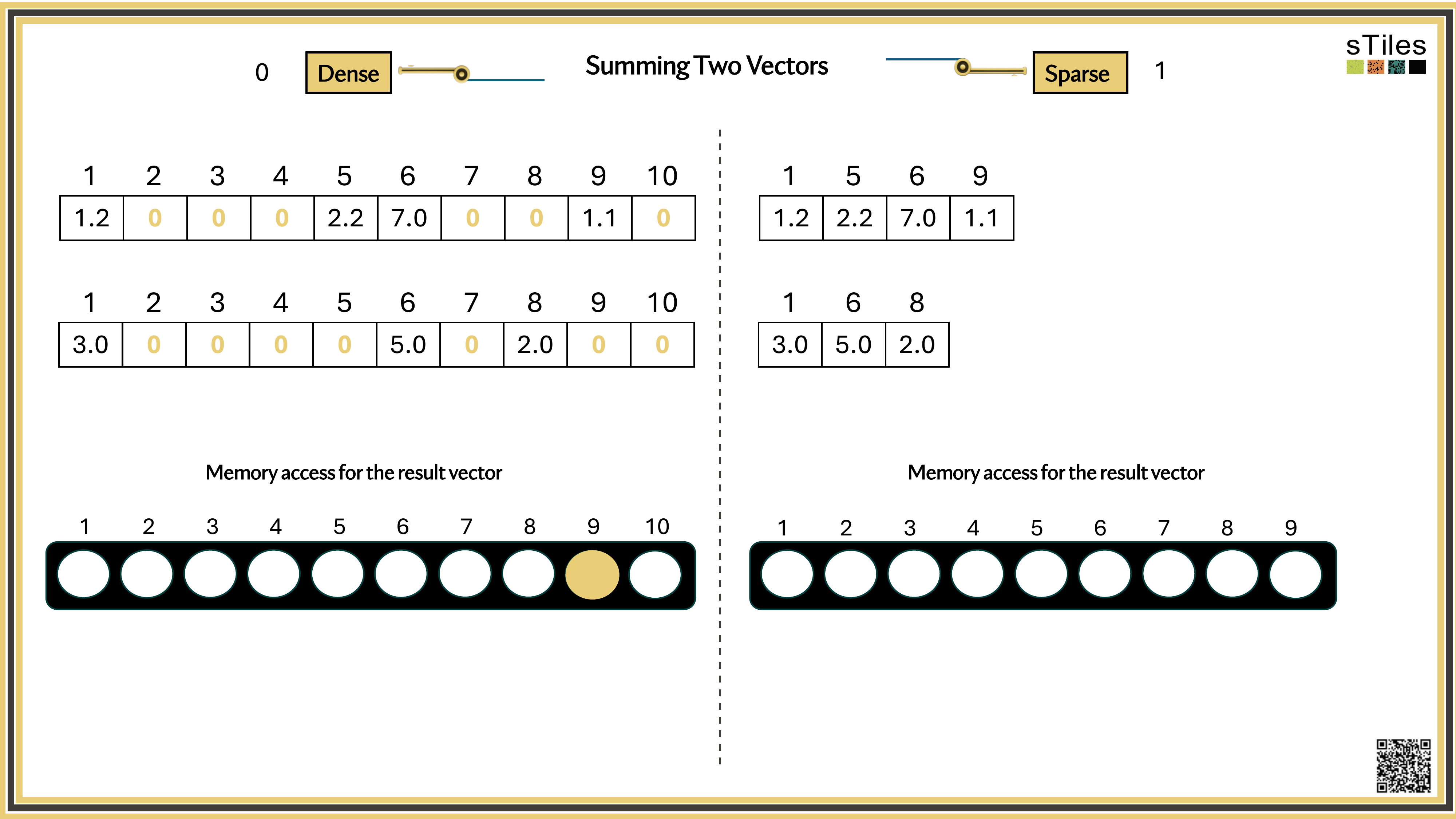
Considers every element of A, even the zeros. Does the same work whether entries are zero or not.
Wastes time on structure it ignores.
Sparse solver
Skips zeros entirely. Only touches non-zero entries, so the work scales with the structure.
Uses the pattern instead of fighting it.
Solving is only half the story.
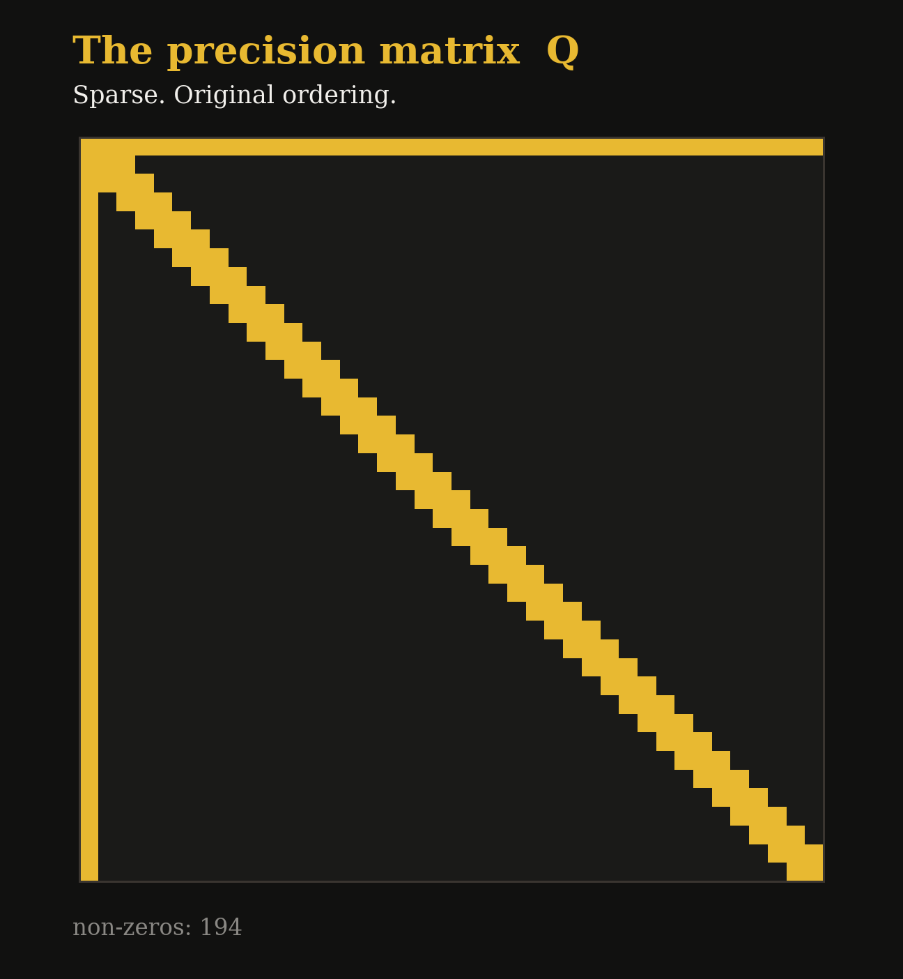
Your model works with a
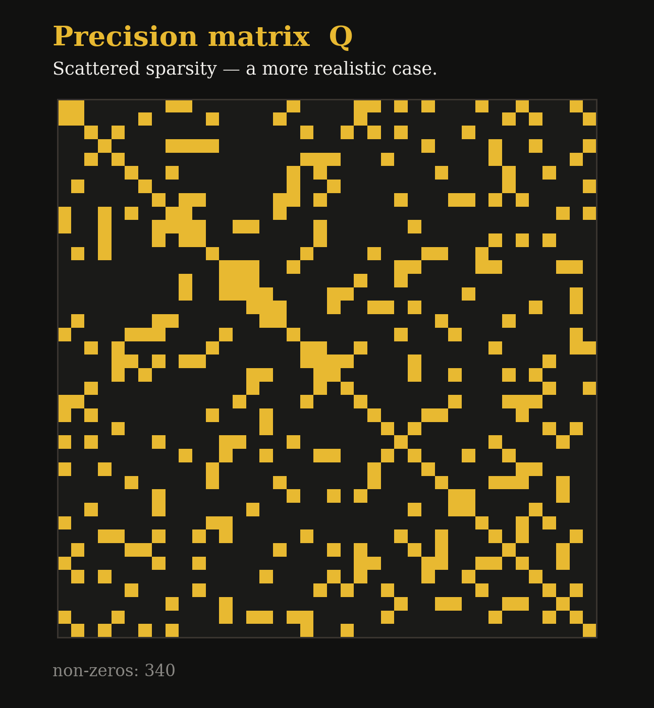
precision matrix Q
Sparse. That's why structured Bayesian and hierarchical methods can scale at all.
But uncertainty lives in the
covariance Σ = Q−1
Dense. Forming it at scale is impossible.
Sometimes you only need
diag(Σ)
One variance per parameter. Selected inversion recovers it from the same Cholesky factor you already computed.
In picture.
What you have, what it inverts to, and what you actually need.
Q
precision (sparse)
Σ = Q−1
covariance (dense)
diag(Σ)
what you need
Selected inversion extracts the gold cells directly from the Cholesky factor, without ever forming the dense Σ.
Why It's Slow · 1 of 2
What makes this step slow?
Size grows fast.
Double the mesh or add a random effect, and Cholesky work grows 4–8×.
Repetition compounds.
Every optimizer step, every hyperparameter, every MCMC iteration triggers another factorization, hundreds to thousands per fit.
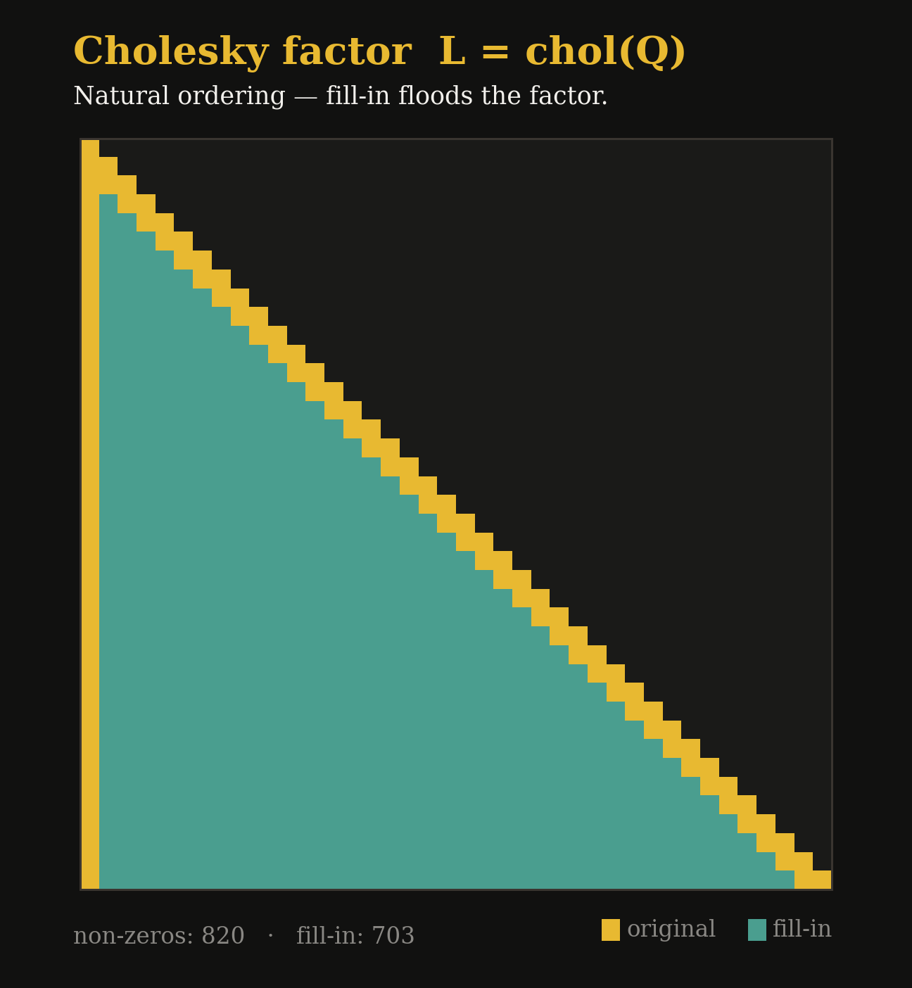
Fill-in explodes.
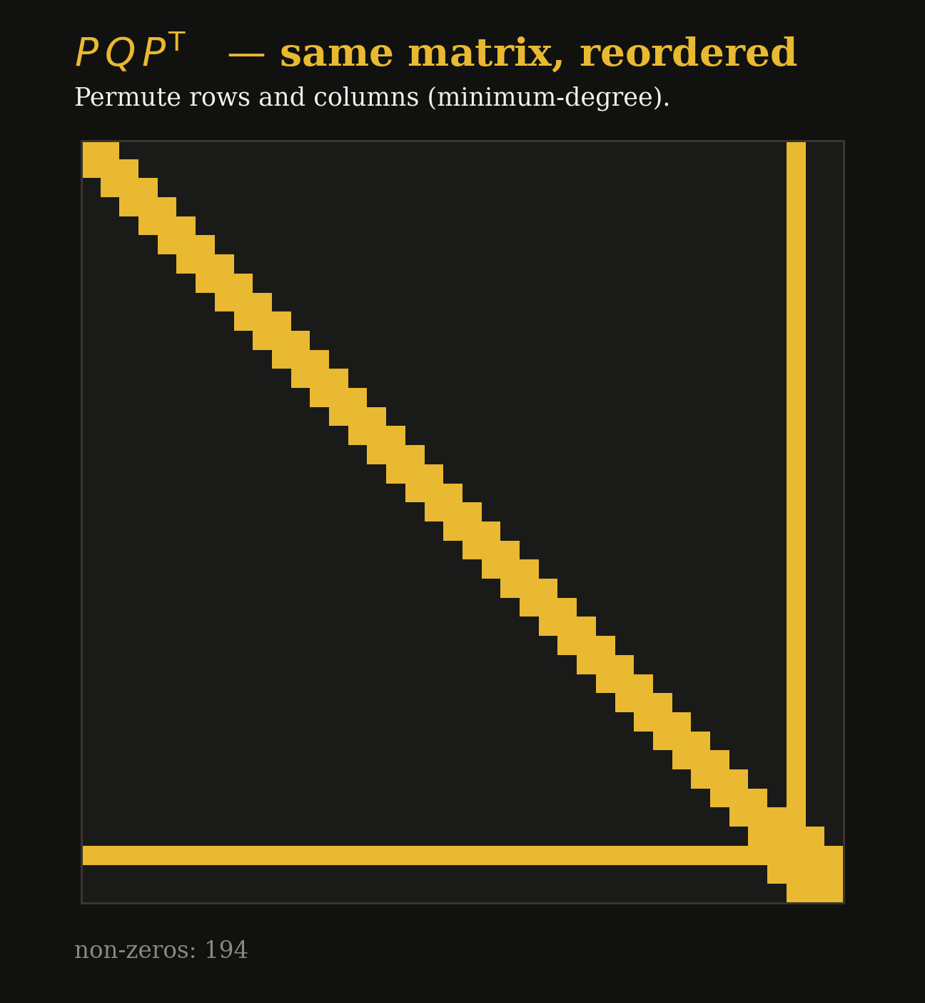
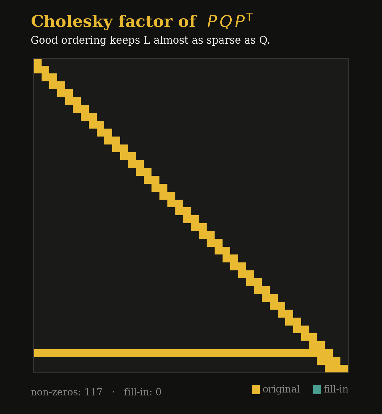
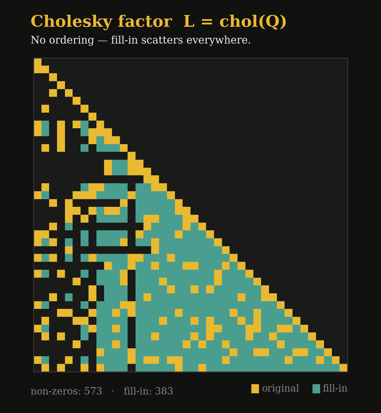
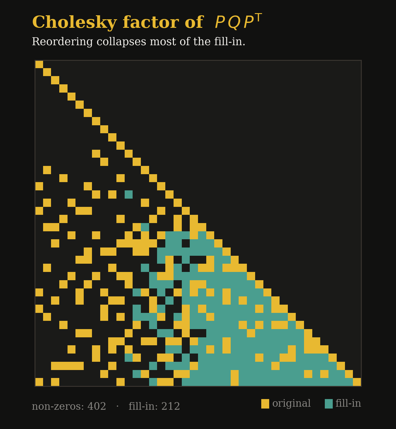
The Cholesky factor is usually far denser than the matrix, often 10–100× more non-zeros if the ordering is poor.
Why It's Slow · 2 of 2
What makes this step slow?
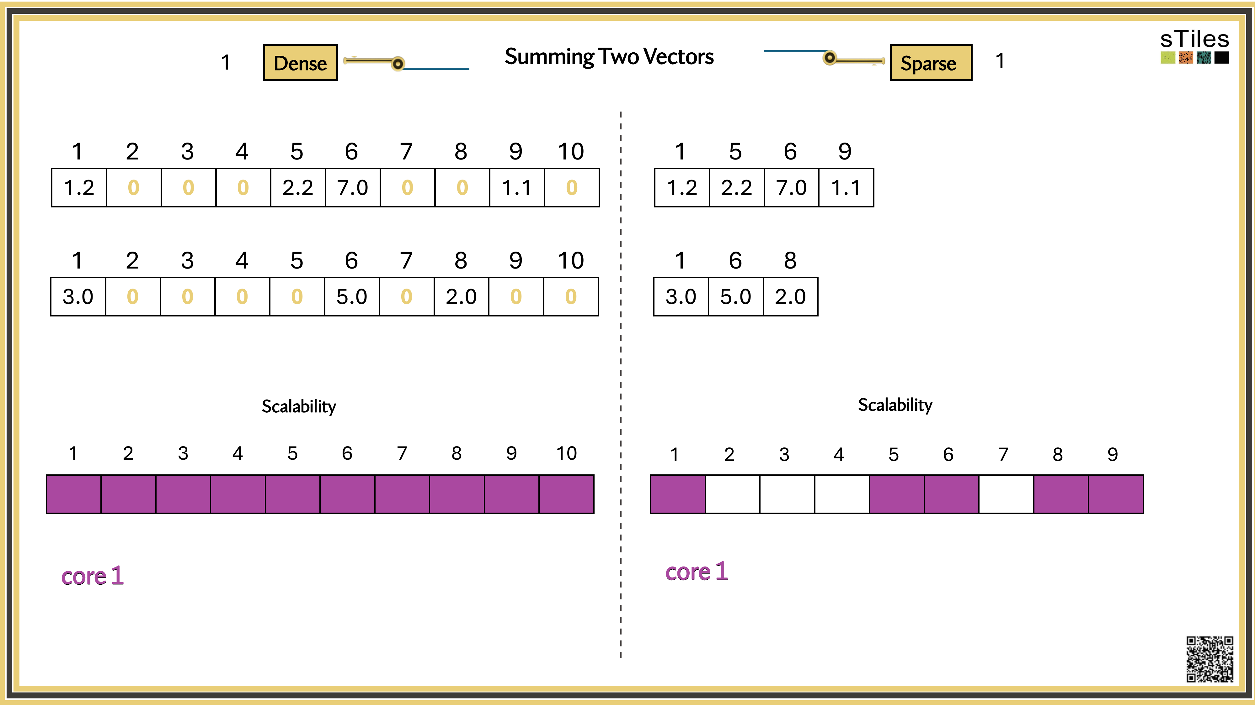
One core by default.
Most solvers pin to a single thread, while your laptop has 8 or more sitting idle.
Memory wall.
Once the factor leaves cache, or RAM, data movement dominates compute.
Understanding the Hardware Behind the Speed
Analogy
CPU
A kitchen with a few expert chefs (the cores), each carefully preparing a complex dish.
GPU
A stadium full of burger flippers, each making the same thing fast and in parallel.
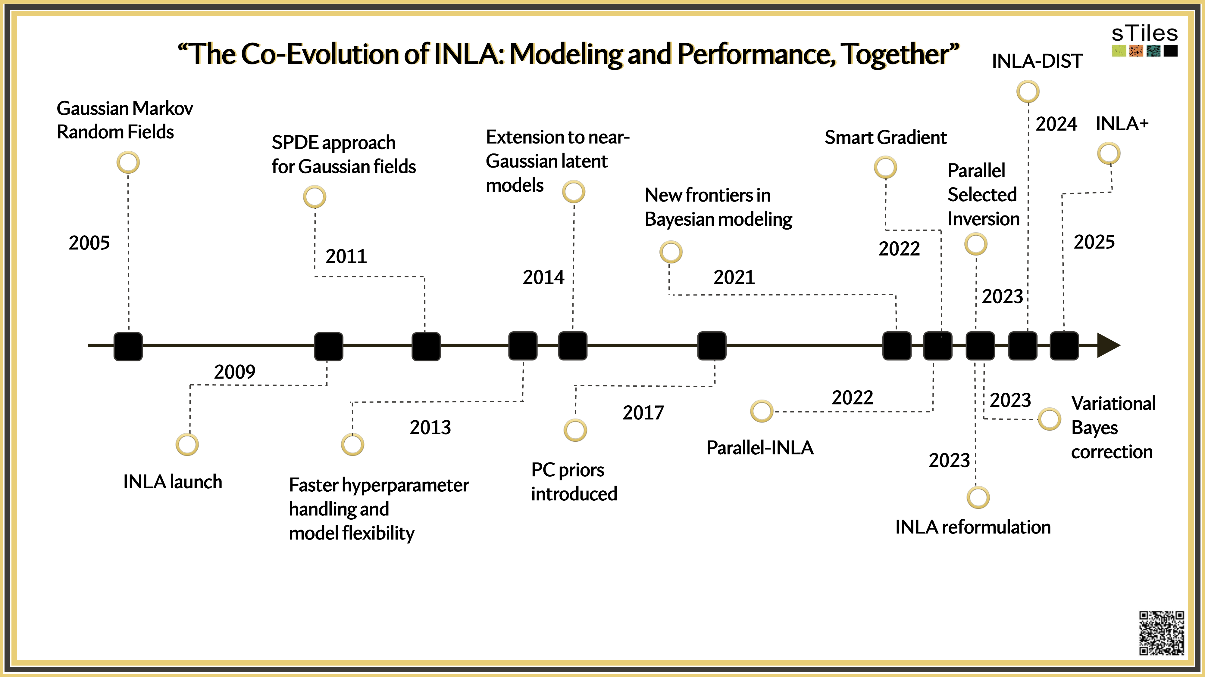
"INLA's computational speed depends not just on clever math, but on how well we use the hardware it runs on."
A complex interaction model* for disease mapping in Spain couldn't be fit using INLA in 2009.
This model took
6 days
to run with default solvers in 2016.
Even in 2024, INLA sometimes crashed or took
hours
to run.
With INLA+, it runs in minutes, reliably.
*Based on: Goicoa et al. (2016), Age-space-time CAR models for Bayesian disease mapping, Stat Med.
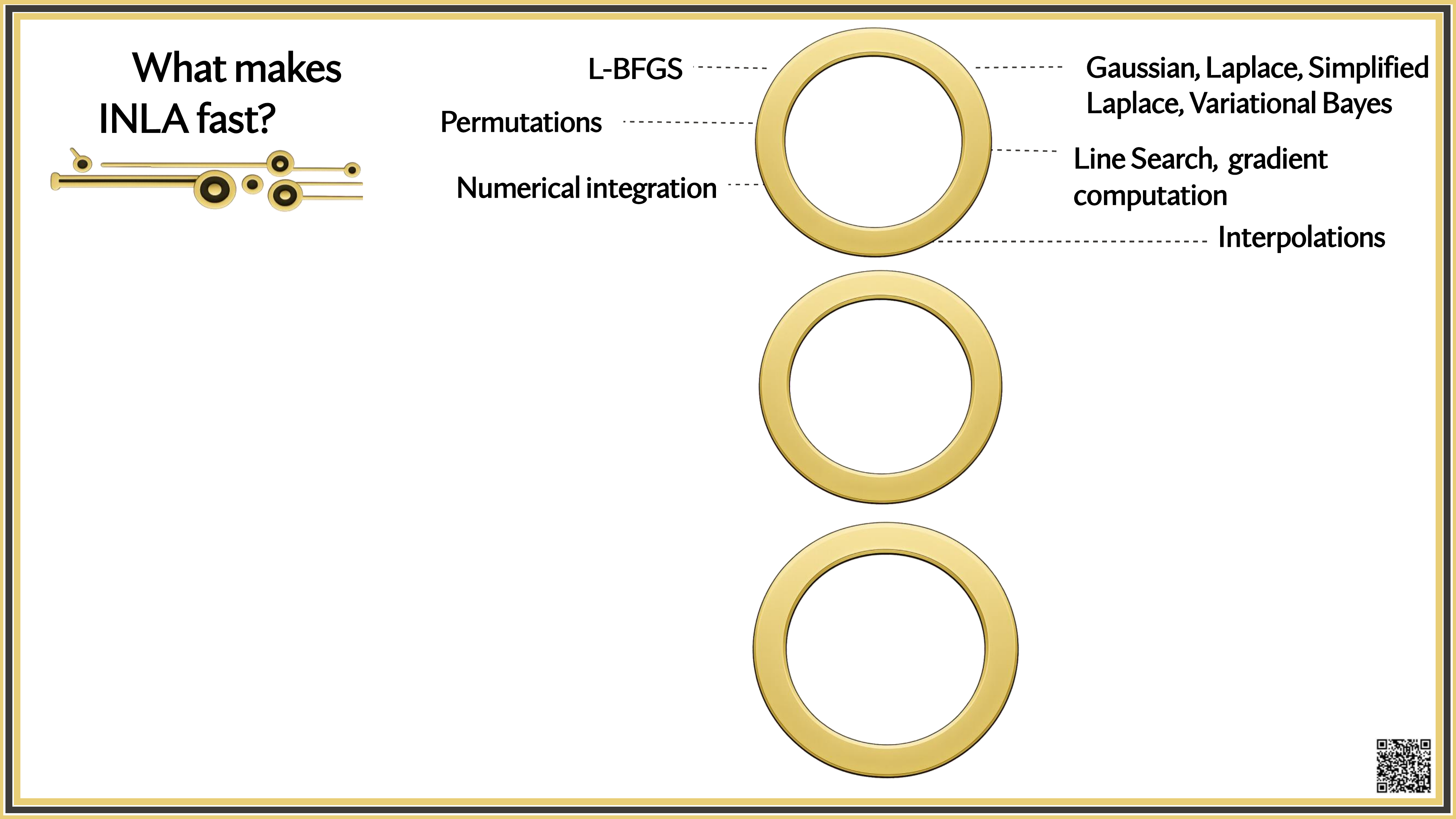
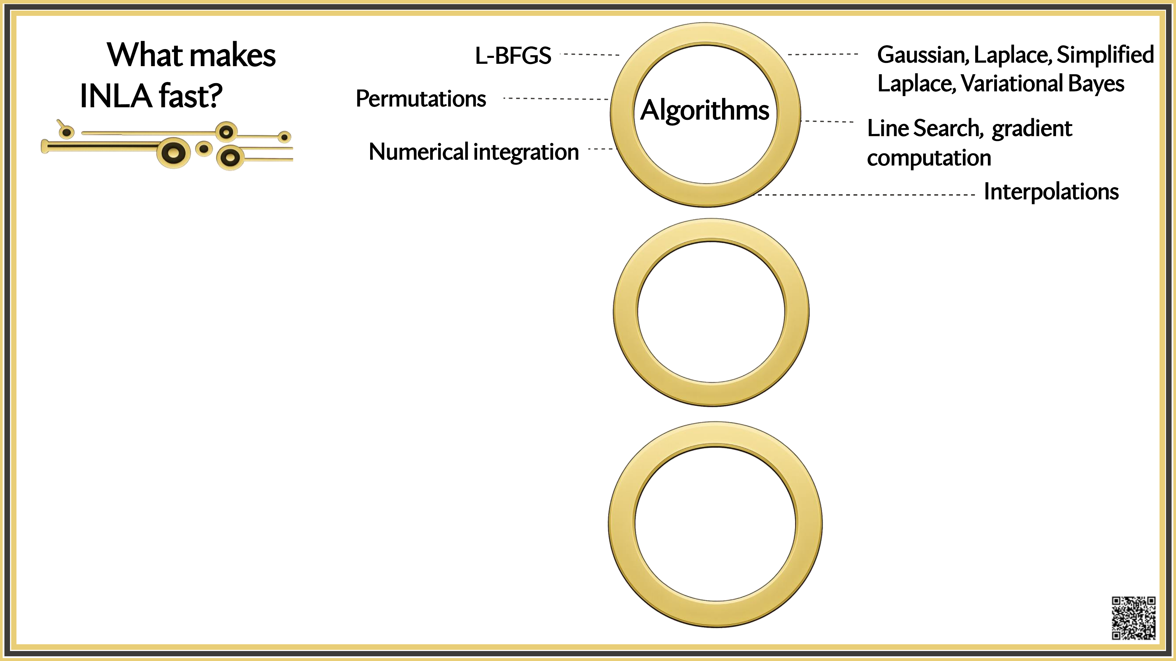
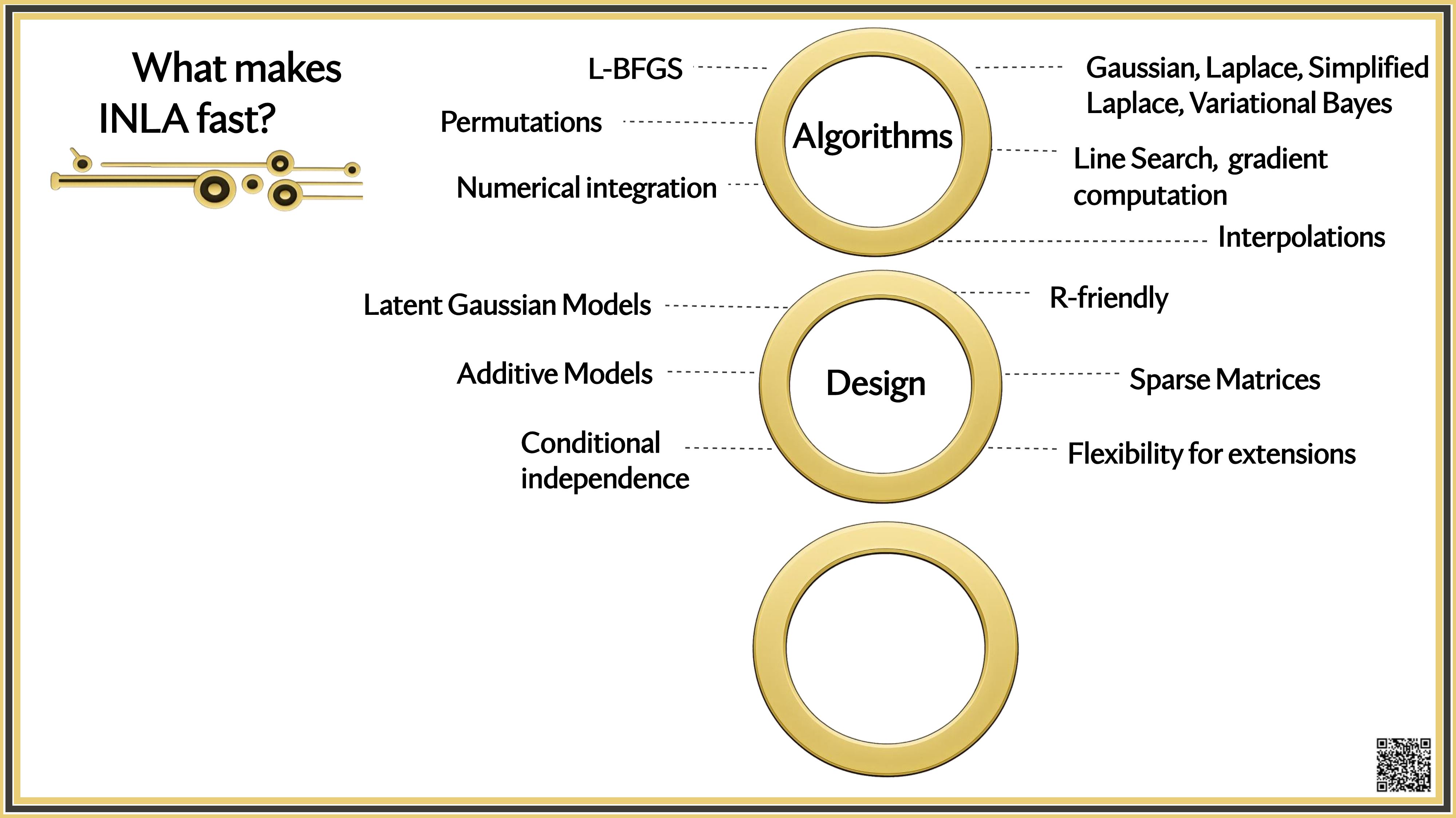
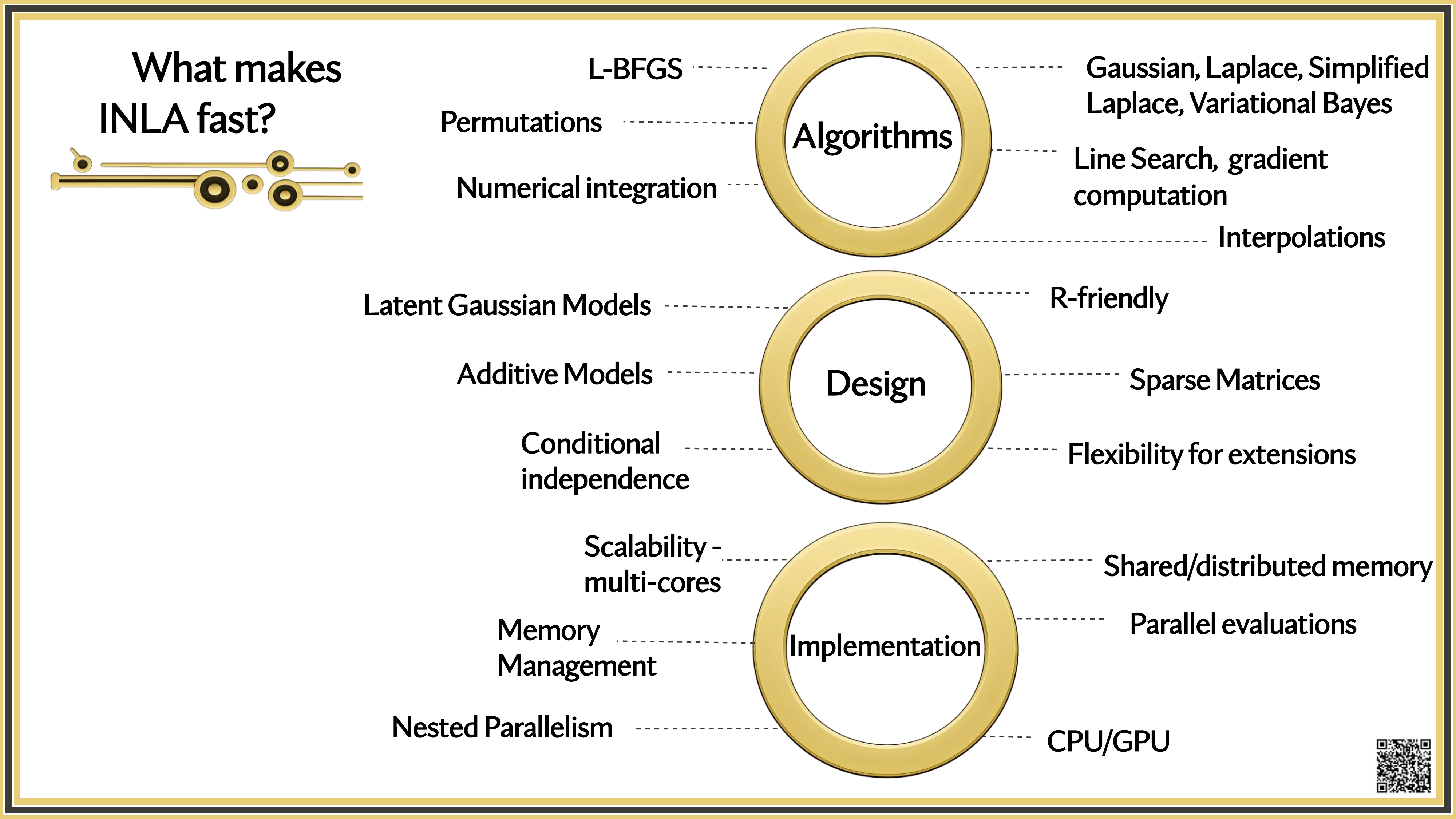
What makes INLA fast?
Is INLA Ready for the Growing Complexity of Models?
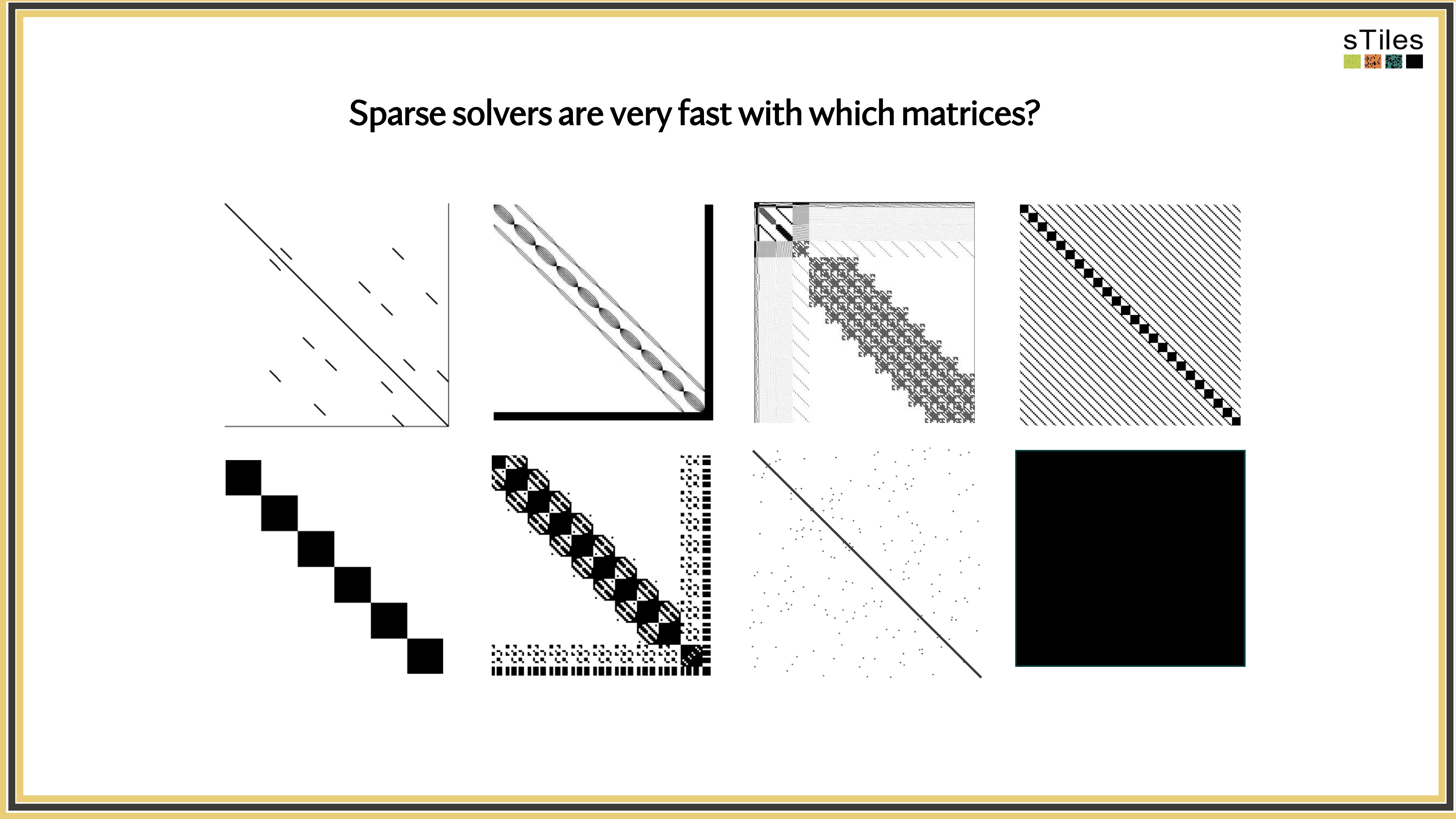
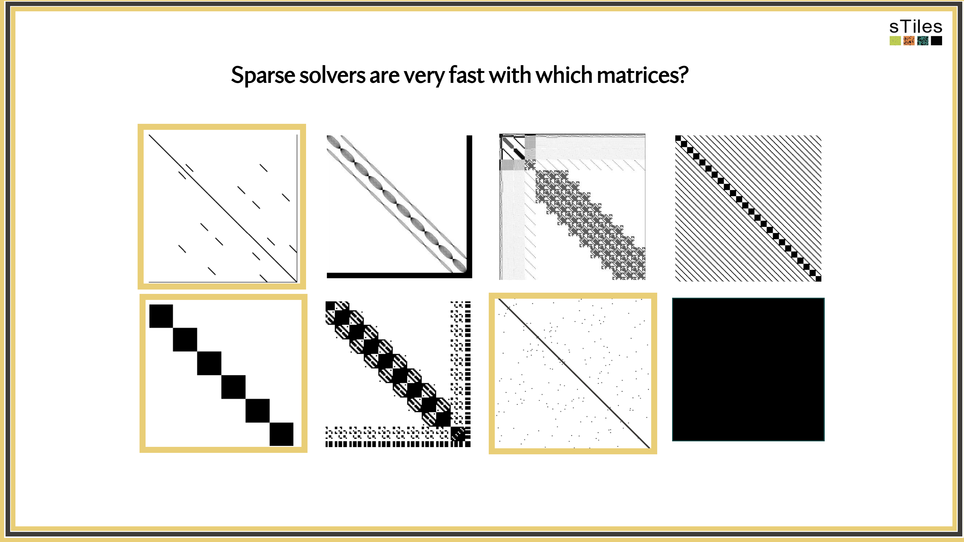
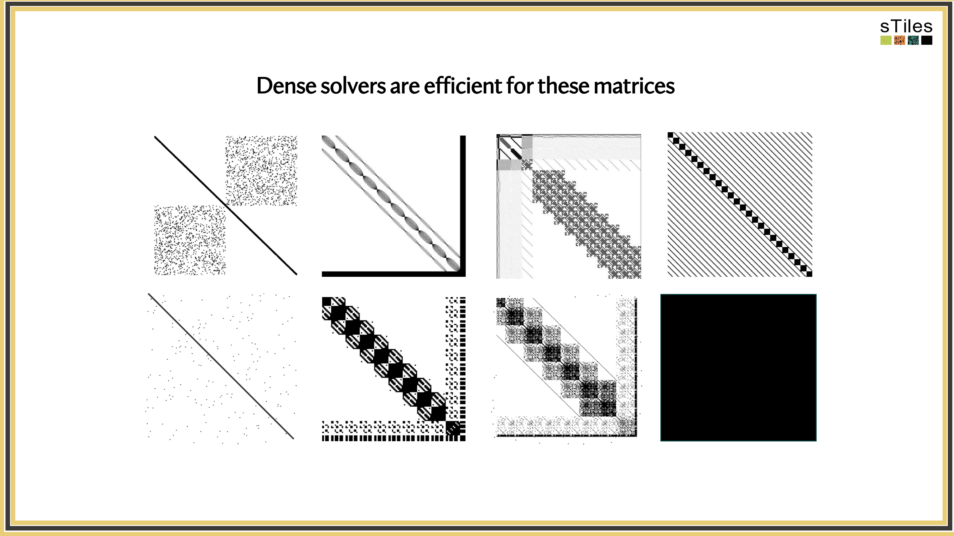
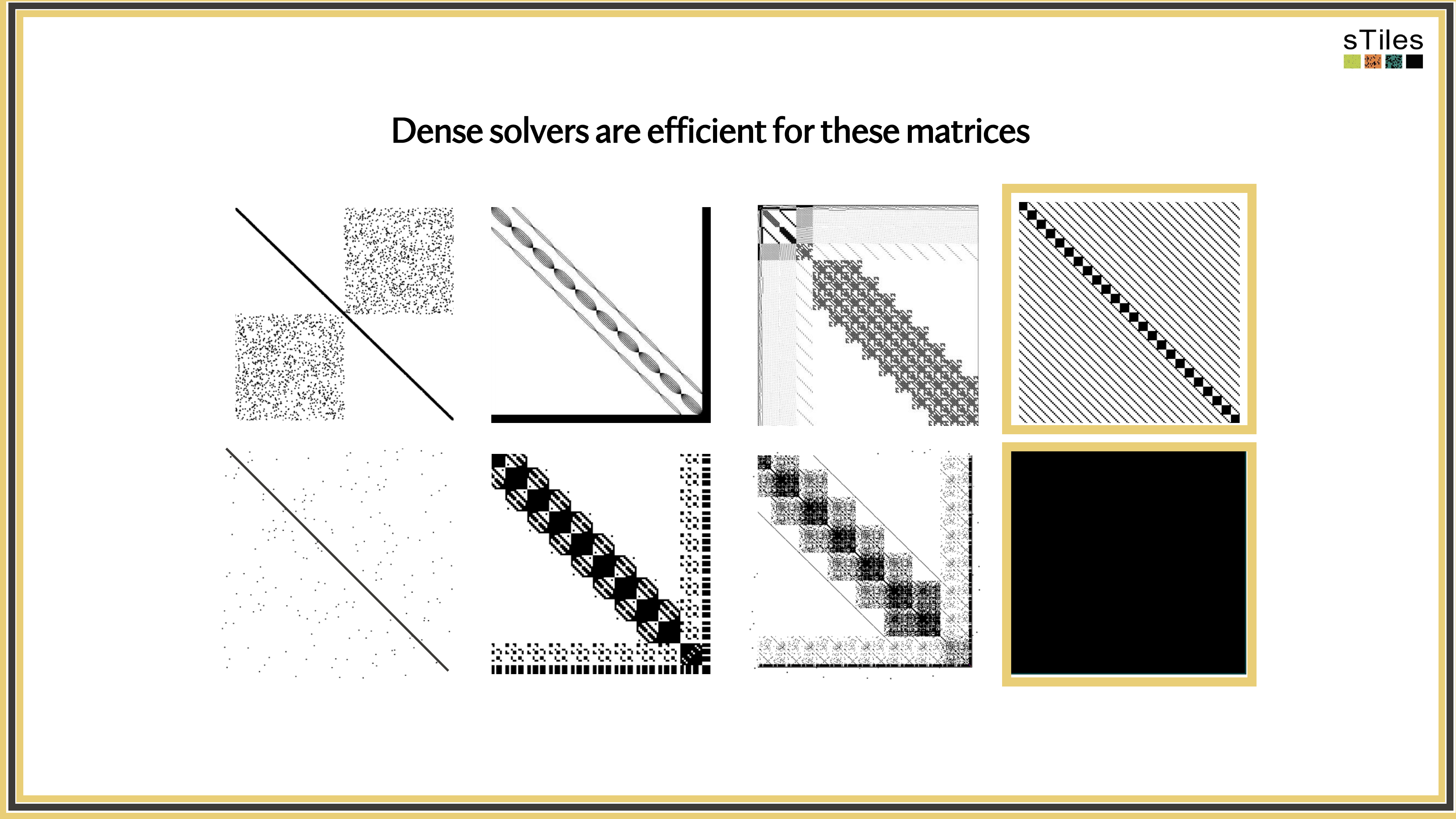
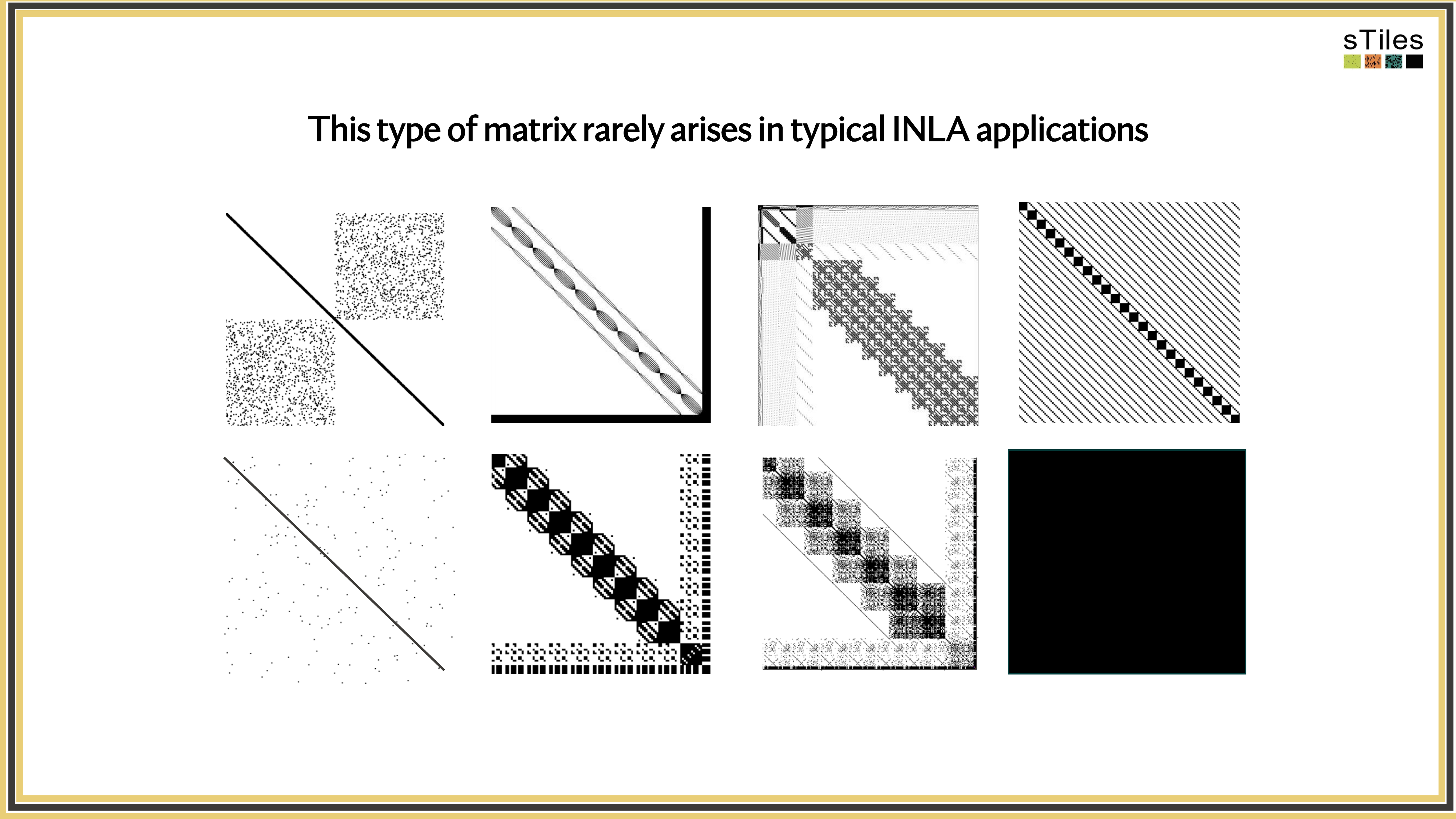
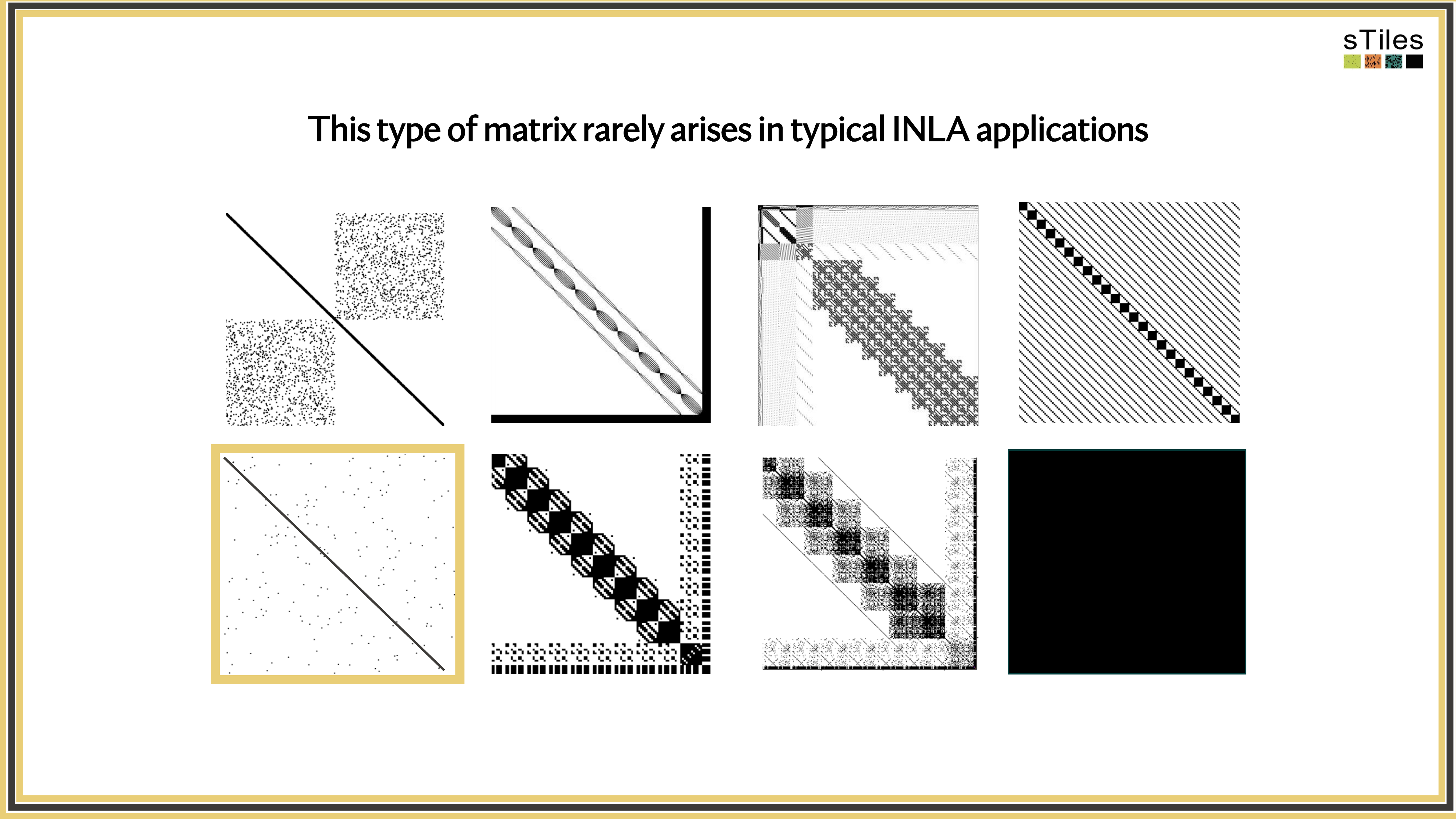
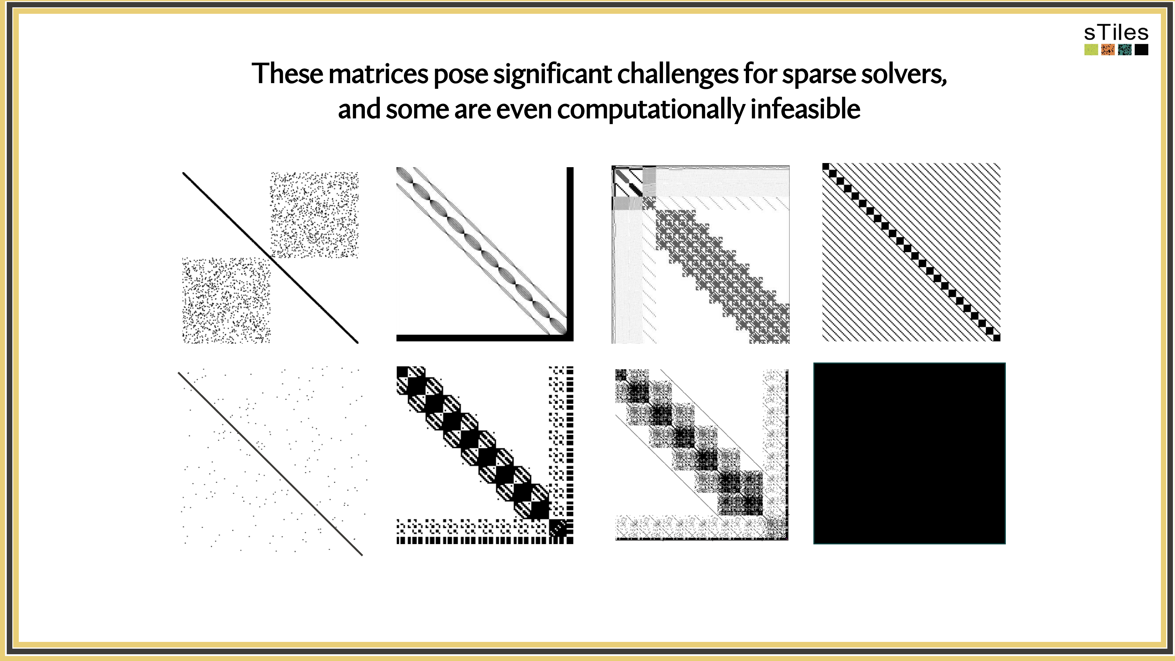
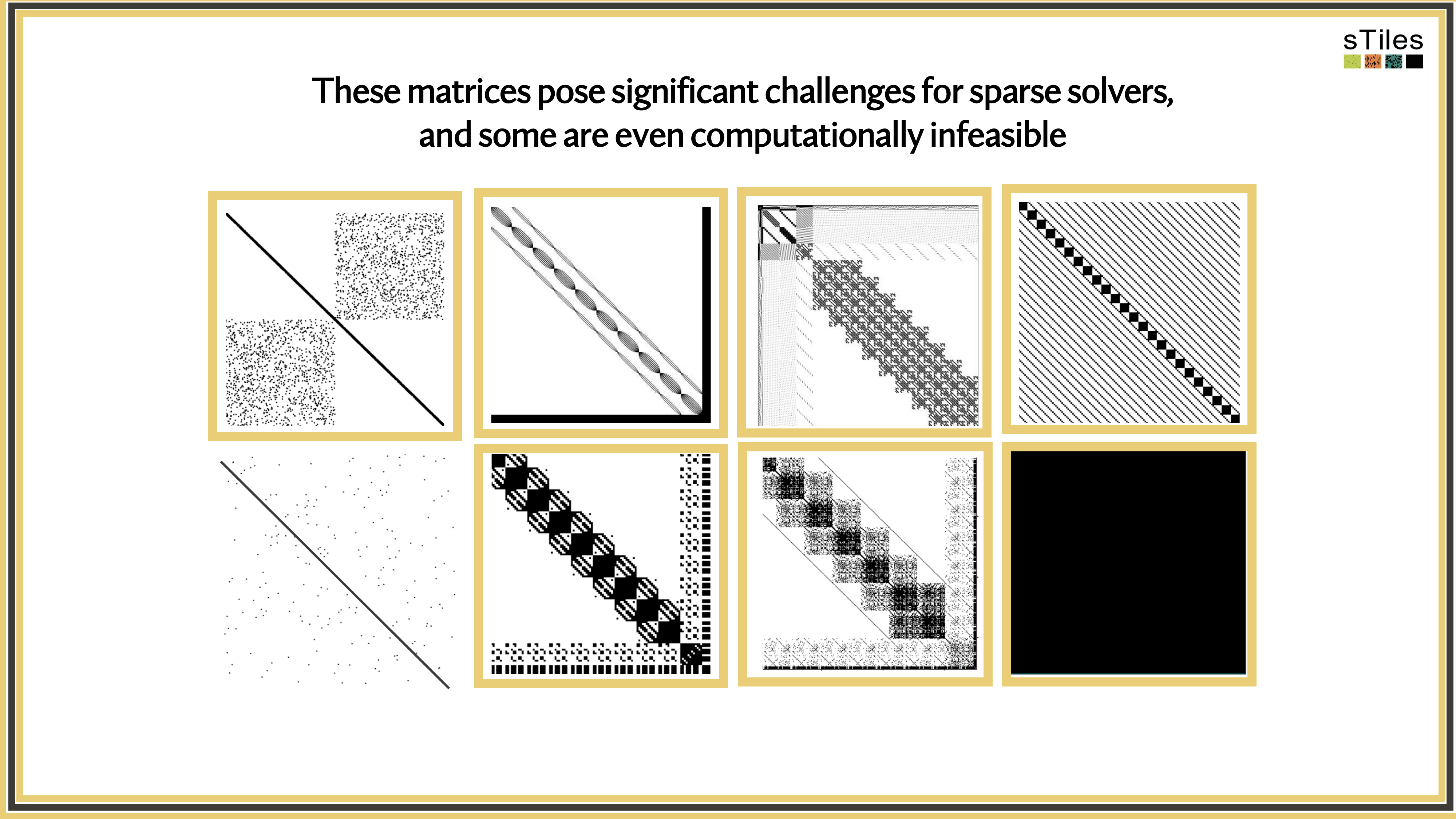
Let's look at what these precision matrices actually look like.
Captcha
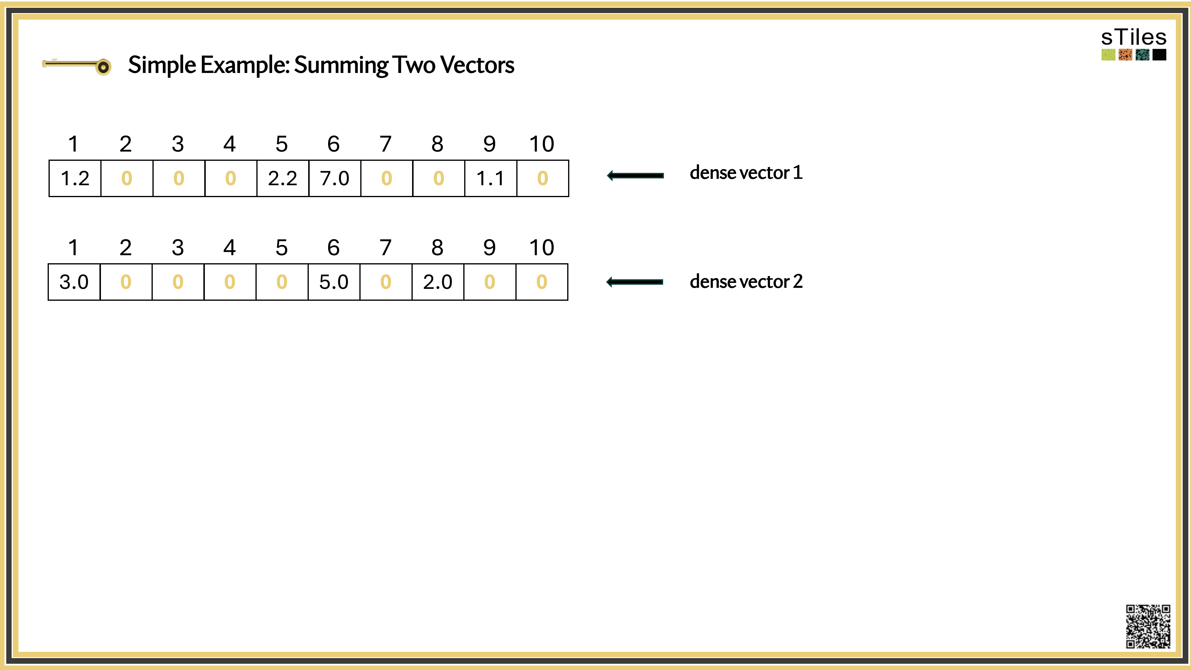
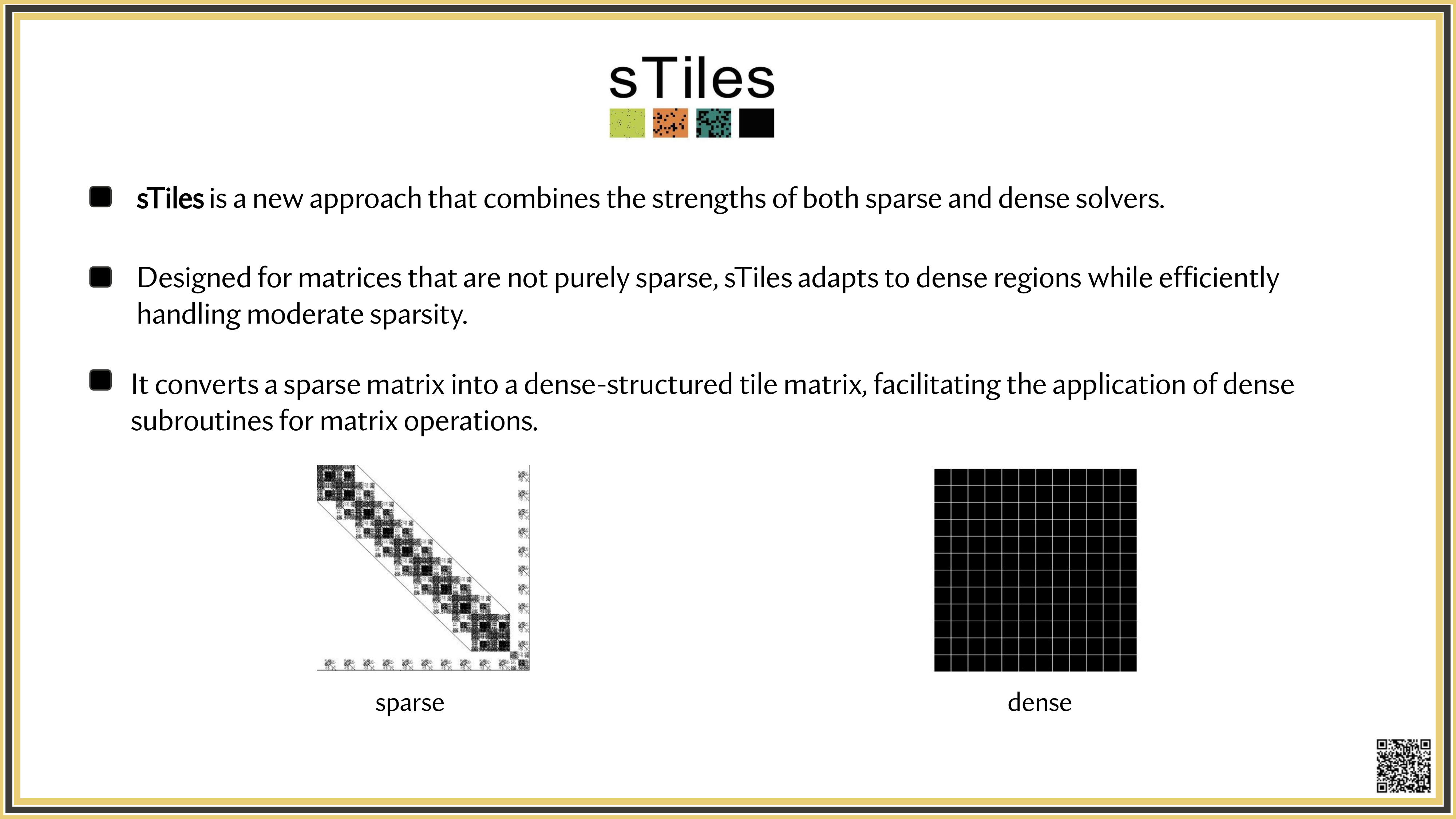
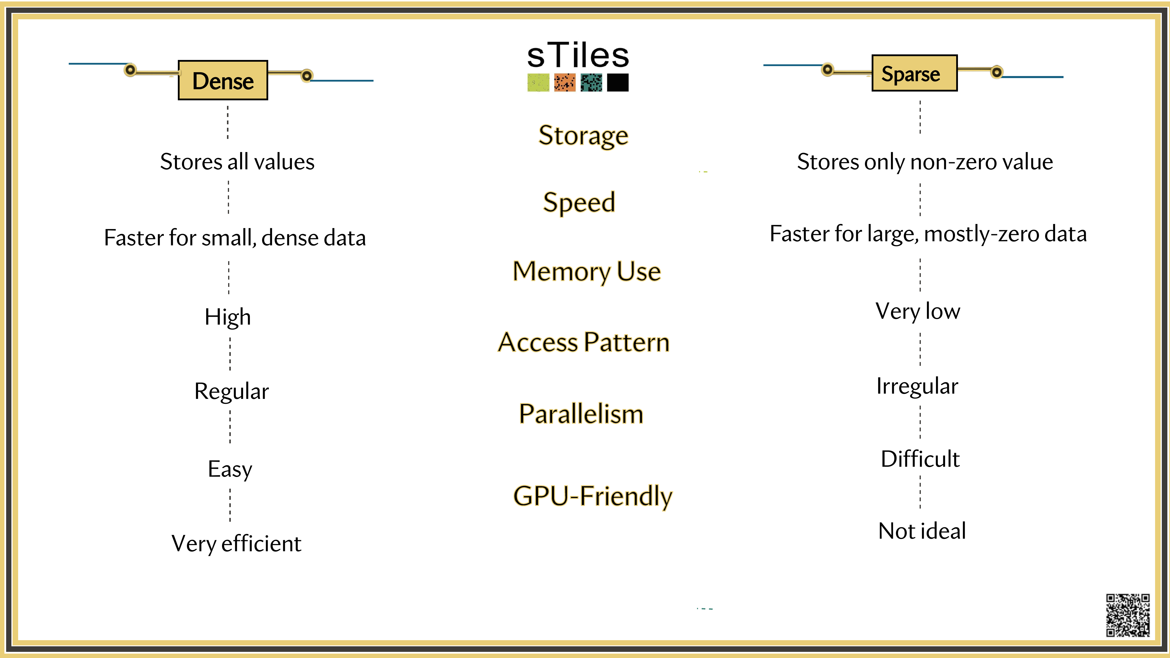
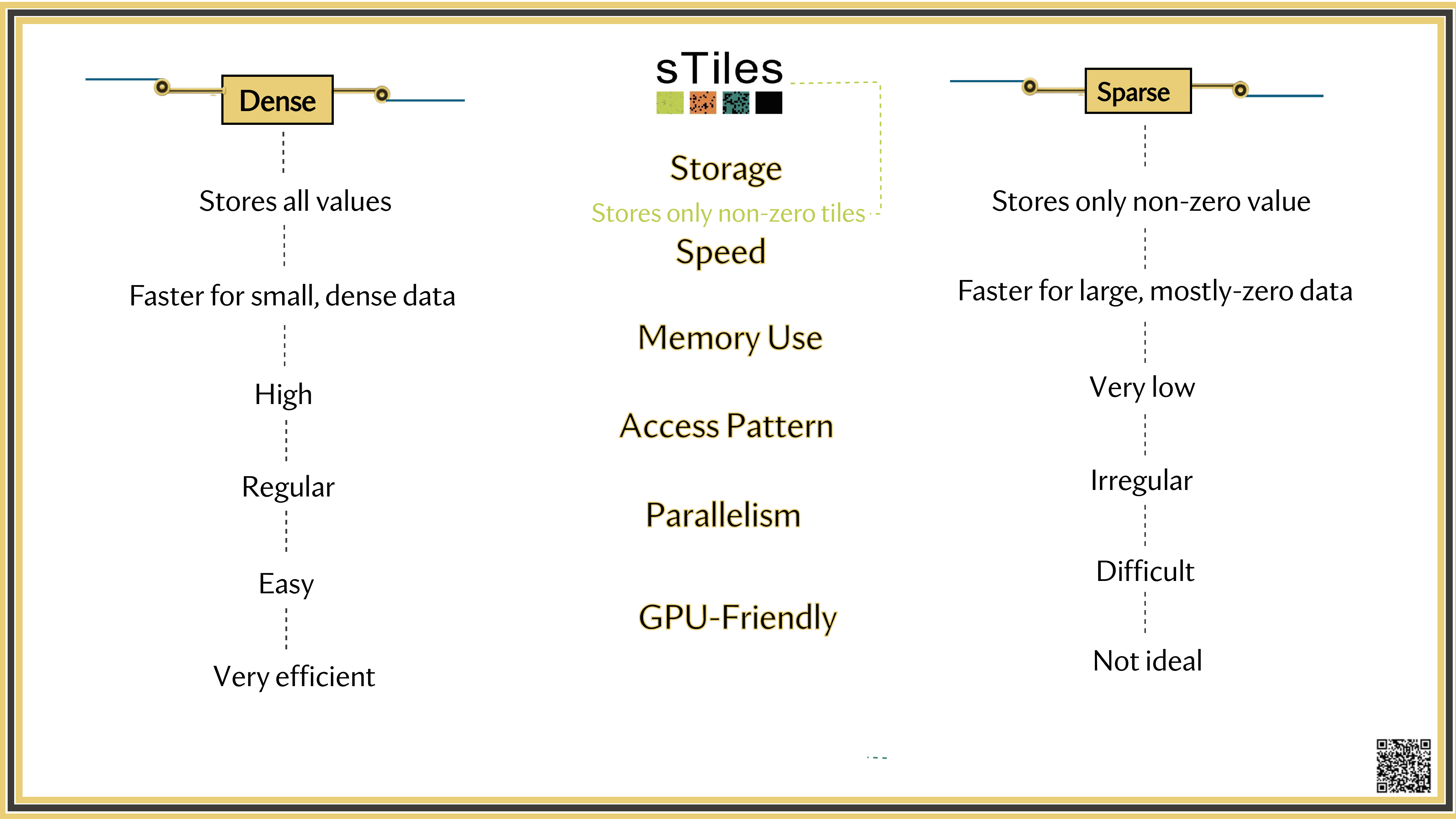
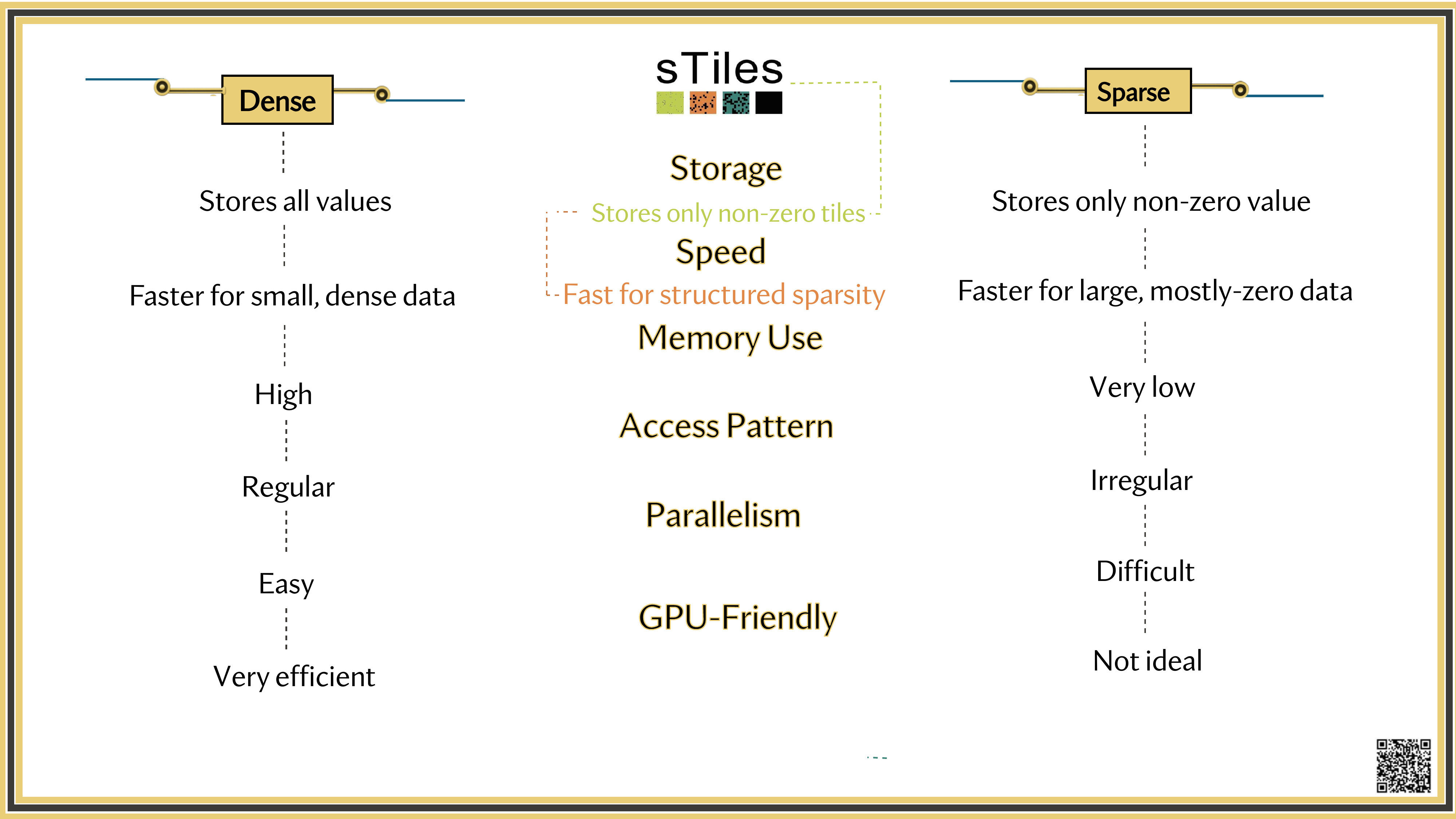
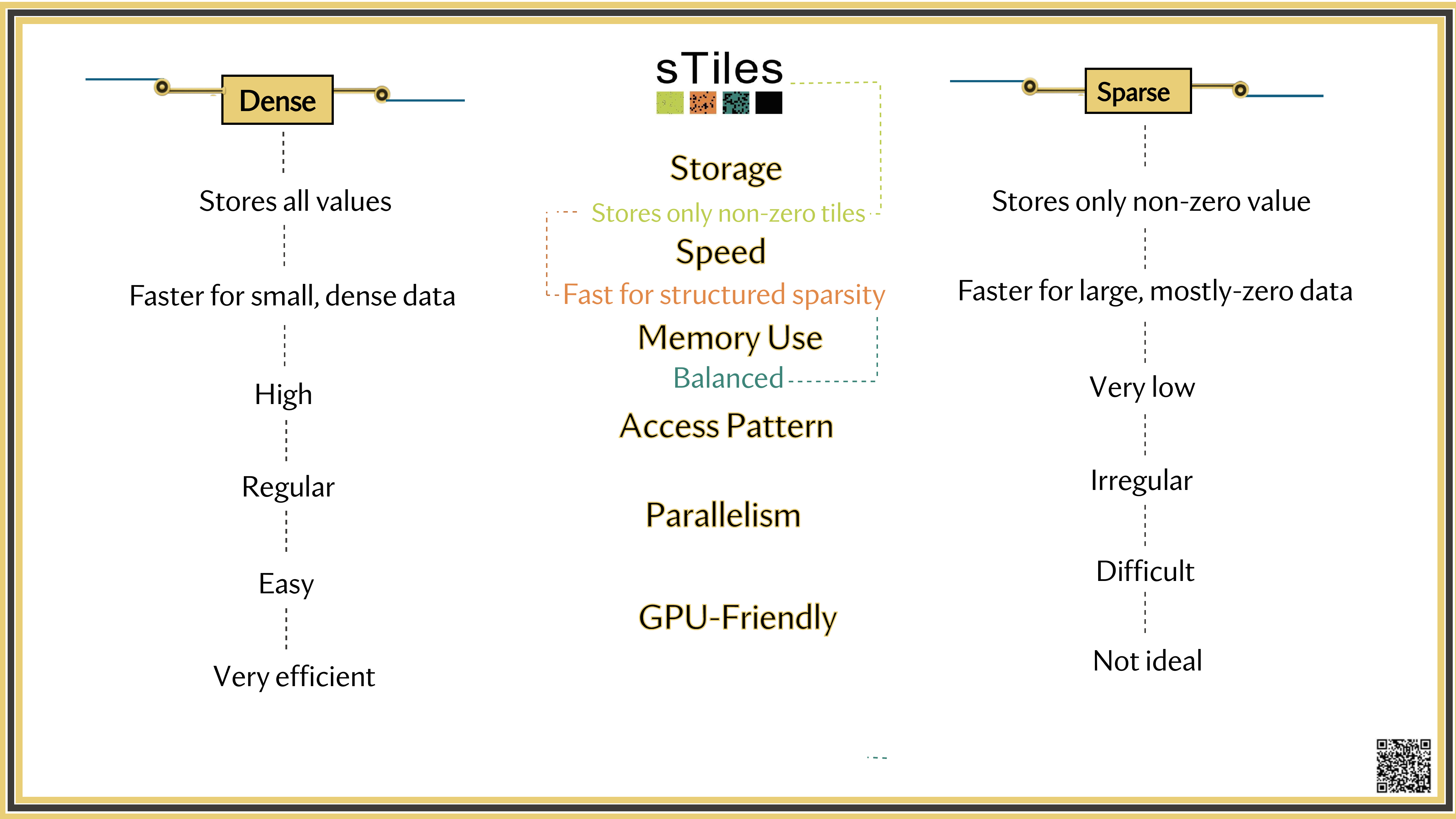
Not All Zeros Are Equal! Sparse vs. Dense
Our Framework
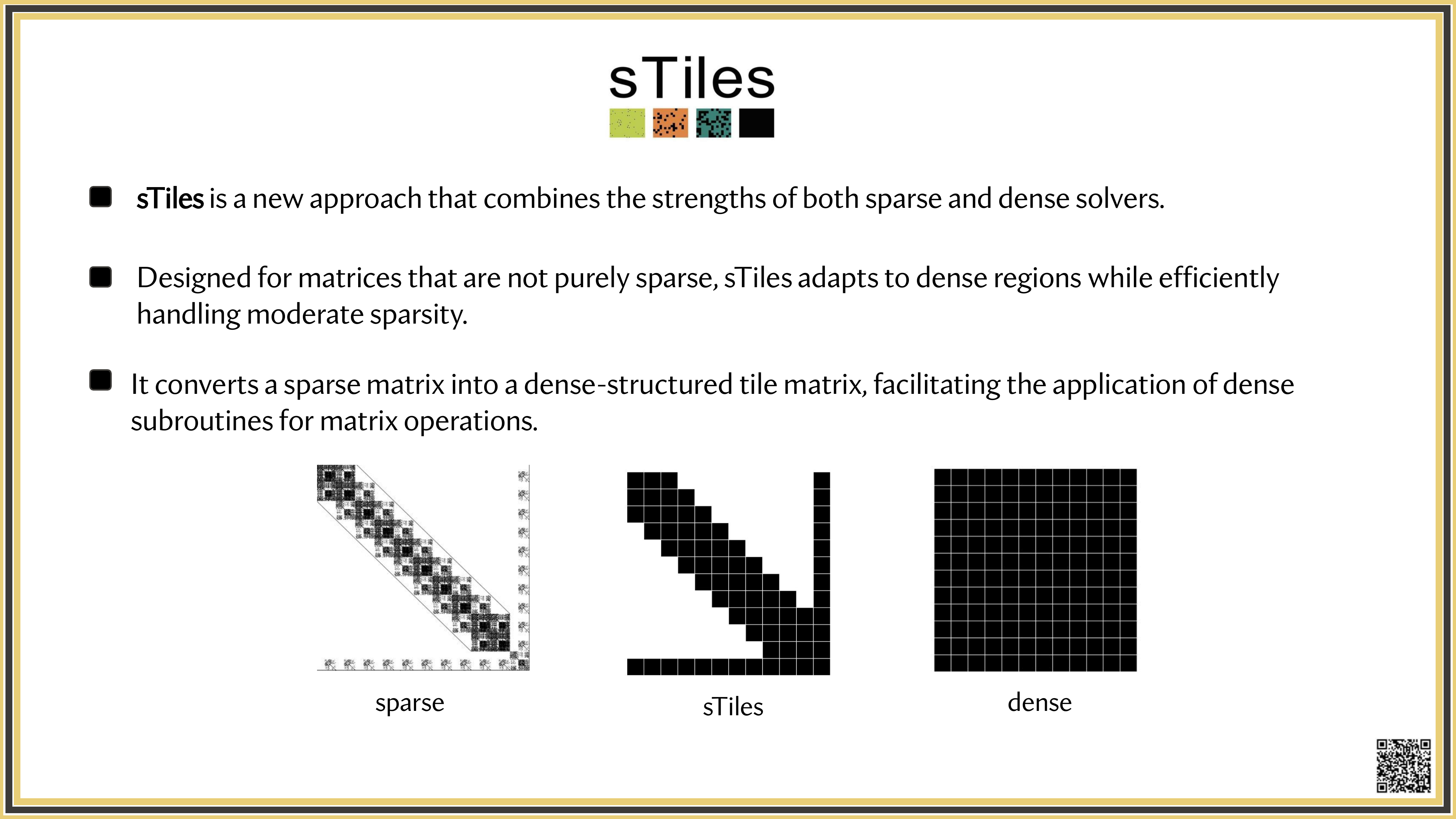
Introducing sTiles
A tile-based hybrid solver: sparse preprocessing, dense performance.
Tile-based linear algebra
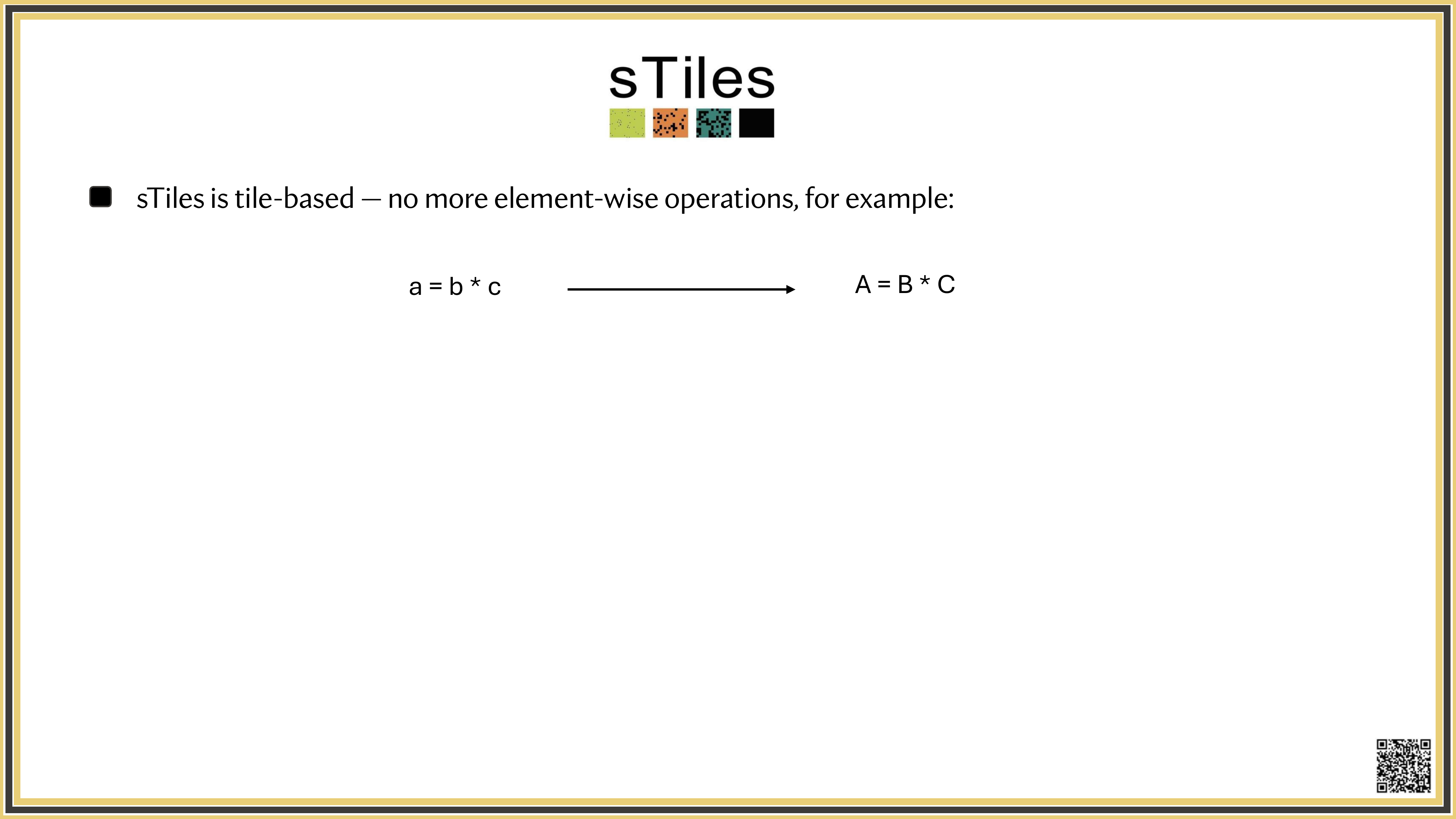
Uniform tiles for sparse + dense compute.
Core idea
Impose a uniform grid of fixed-size tiles on the matrix. Regular data, predictable dependencies.
Why tiles?
Finer granularity — more parallel tasks
Cache locality — each tile fits in cache
BLAS-3 kernels — GEMM, TRSM, POTRF on every tile
Static schedule — no runtime overhead, GPU-ready
Traditional supernodal
Variable block sizes
Irregular data structures
Dynamic scheduling
Hard to optimize for GPUs
sTiles
Fixed tile sizes (tunable)
Regular data structures
Static, pre-computed schedule
One codebase, CPUs and GPUs
What you'll see next
The same matrices you've been fighting with, fitted faster.
So, What's Slowing You Down?
Adding interactions or finer resolution doesn't just add rows.
It changes the
matrix structure
sometimes dramatically.
If each run takes an hour, you try 4 a day.
If it takes 2 minutes, you try 50.
Speed changes the science
not just the wait.
Don't simplify your science for your computer.
The real fix is a better solver, not a worse model.