Selected Inversion

GPU-Accelerated Parallel Algorithms for Structured Sparse Matrices

Esmail Abdul Fattah

esmail.abdulfattah@kaust.edu.sa

King Abdullah University of Science and Technology

Hatem Ltaief, Håvard Rue, David E. Keyes

SIAM PP26 · March 2026

Introduction

What is Selected Inversion?

Computing only the inverse elements that matter

Problem

Given a sparse matrix A, we need specific elements of A-1. However, the full inverse is typically dense, making direct computation prohibitive.

A · A-1 = I

Key Idea

Compute only (A-1)ij where Aij ≠ 0, preserving the sparsity pattern.

A (sparse) Tiled arrowhead invert A-1 (full) 36 entries (dense!) select A-1 (selected) 16 entries only! Pattern of A = Pattern of Selected A-1 56% savings Nonzero Tile boundary Dense fill (avoid)

Motivation

Real-World Arrowhead Matrices

Different sparsity levels, same selected inverse structure

Matrix A (sparse)

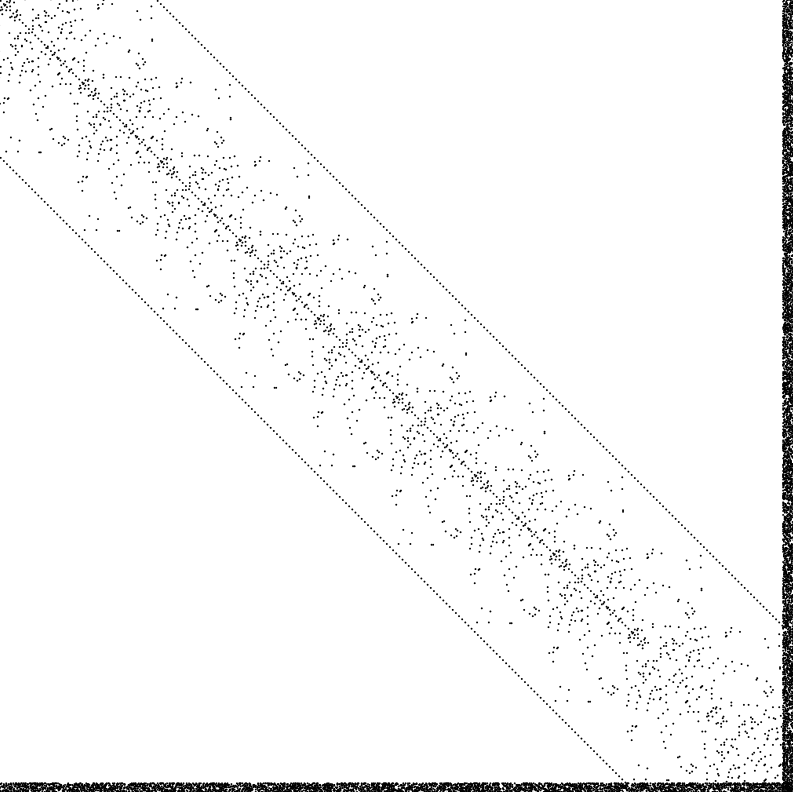
Few spatial locations

Matrix B (denser)
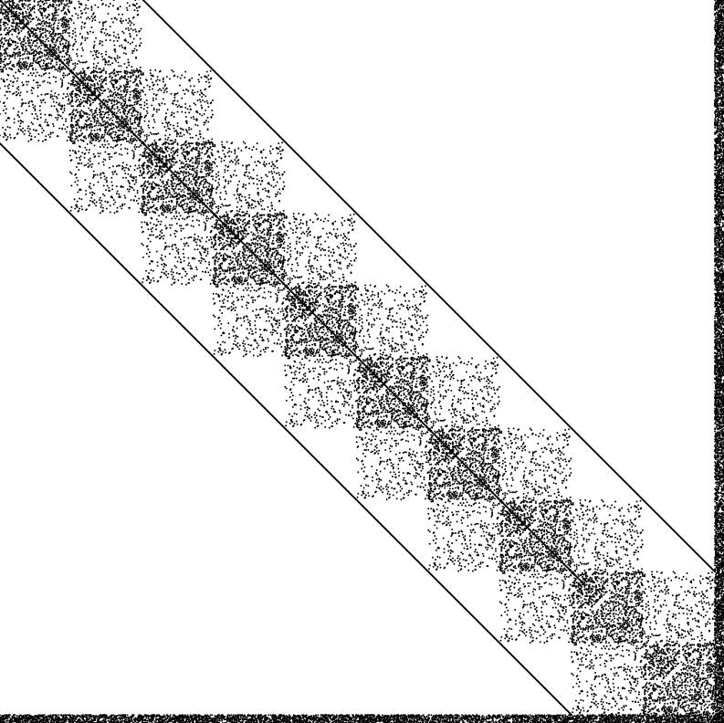
More spatial locations

Selected Inverse

Same dense arrowhead!

Same dense arrowhead!

Key Observation

Regardless of initial sparsity, the selected inverse retains the arrowhead structure. This enables efficient tile-based computation.

Why Arrowhead Structure?

Arrowhead matrices arise from Kronecker products modeling space-time dependencies:

  • Spatio-temporal models
  • Gaussian Markov Random Fields
  • Hierarchical Bayesian models

Real Applications
WHO mortality CDC disease UN demographics Climate

Data Structure

Tile Mapping

From scalar indices to contiguous tile storage

(i, j) Scalar (k, m) Tile Linear Storage 0 1 2 3 4 5 ...

Scalar Index

Element position in matrix

Tile Index

Tile containing element

Linear Storage

Contiguous memory layout

Why This Matters

Tiles are stored contiguously in memory, enabling cache-efficient BLAS-3 operations and predictable memory access patterns.

Core Concept

How Selected Inversion Works

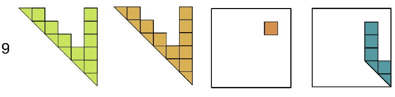
Dense Matrices (1-5)
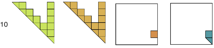
Arrowhead Matrices (6-10)
Matrix A
Cholesky
Selected Tiles
Inversion
full → full
diag → full!
diag+ → full!
off-diag → min
corner → min
Matrix A
Cholesky
Selected Tiles
Inversion
full → full
arrow → arrow! ★
partial → partial
off-diag → min
corner → min
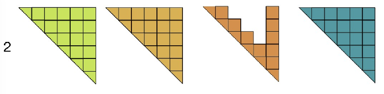
Case 1: Full selection on dense matrix → requires computing the entire inverse. Maximum cost.
Cases 2-3: Selecting only diagonal tiles still requires full inverse! The diagonal depends on ALL off-diagonal elements.
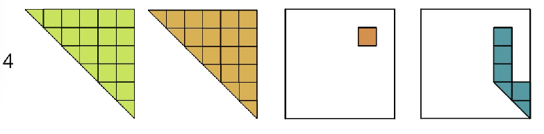
Cases 4-5: Selecting off-diagonal without diagonal → minimal computation needed. Only selected element + corner.
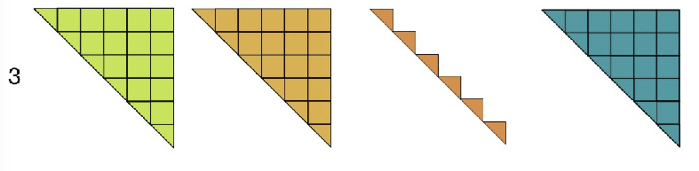
Cases 6-8 (Arrowhead): Case 7 is key! Arrowhead selection on arrowhead matrix preserves structure → inverse stays arrowhead!
Cases 9-10: Like dense cases 4-5, selecting off-diagonal without diagonal → minimal computation.
Key Insight: For INLA: arrowhead matrices with arrowhead selection (Case 7) → huge savings! Our algorithm exploits this structure.

Algorithm

Tile-Based Inversion

3×3 tiled matrix example: LTΣ = L-1

Σ (inverse) Σ₀₀ Σ₁₁ Σ₂₂ Σ₁₀ Σ₂₀ Σ₂₁ L (Cholesky) L₀₀ L₁₀ L₁₁ L₂₀ L₂₁ L₂₂ 0 0 0
Recursive equations (bottom-right → top-left):
Σ₂₂ = L₂₂-T L₂₂-1
Σ₂₁ = -Σ₂₂ L₂₁ L₁₁-1
Σ₁₁ = L₁₁-T L₁₁-1 - L₁₁-T L₂₁T Σ₂₁
Σ₂₀ = -Σ₂₁ L₁₀ L₀₀-1 - Σ₂₂ L₂₀ L₀₀-1
Σ₁₀ = -Σ₁₁ L₁₀ L₀₀-1 - Σ₁₂ L₂₀ L₀₀-1
Σ₀₀ = L₀₀-T L₀₀-1 - L₀₀-T L₁₀T Σ₁₀ - L₀₀-T L₂₀T Σ₂₀

Σ (inverse)

Σ₀₀ Σ₁₀ Σ₁₁ Σ₂₀ Σ₂₁ Σ₂₂ Σ₂₂ Σ₂₁ Σ₁₁ Σ₂₀ Σ₁₀ Σ₀₀
Computing Σ₂₂ Computing Σ₂₁ Computing Σ₁₁ Computing Σ₂₀ (∥ with ③) Computing Σ₁₀ Computing Σ₀₀

Anti-Diagonal Parallelism

Level 3: Σ₁₁ and Σ₂₀ on same anti-diagonal → no mutual deps → run in parallel!

Parallelization

Two-Phase Parallel Algorithm

3×3 tiled matrix example

P1 Phase 1: Diagonal Blocks ∥ PARALLEL

Σ₂₂ = L₂₂-T L₂₂-1
Σ₁₁ = L₁₁-T L₁₁-1
Σ₀₀ = L₀₀-T L₀₀-1

Phase 2: Off-diagonal + Updates

L1 Σ₂₁ = -Σ₂₂ L₂₁ L₁₁-1
L2
Σ₁₁ += - L₁₁-T L₂₁T Σ₂₁
Σ₂₀ = -Σ₂₁ L₁₀ L₀₀-1 - Σ₂₂ L₂₀ L₀₀-1
L3 Σ₁₀ = -Σ₁₁ L₁₀ L₀₀-1 - Σ₁₂ L₂₀ L₀₀-1
L4 Σ₀₀ += - L₀₀-T L₁₀T Σ₁₀ - L₀₀-T L₂₀T Σ₂₀

Complete Recursive Equations

Σ₂₂ = L₂₂-T L₂₂-1
Σ₂₁ = -Σ₂₂ L₂₁ L₁₁-1
Σ₁₁ = L₁₁-T L₁₁-1 - L₁₁-T L₂₁T Σ₂₁
Σ₂₀ = -Σ₂₁ L₁₀ L₀₀-1 - Σ₂₂ L₂₀ L₀₀-1
Σ₁₀ = -Σ₁₁ L₁₀ L₀₀-1 - Σ₁₂ L₂₀ L₀₀-1
Σ₀₀ = L₀₀-T L₀₀-1 - L₀₀-T L₁₀T Σ₁₀ - L₀₀-T L₂₀T Σ₂₀

sTiles Optimization

  • Skip zero tiles: only compute selected pattern
  • Static scheduling: tasks pre-assigned per core
  • No runtime overhead: task list computed once

Σ (inverse) - Parallel Execution

Σ₀₀ Σ₁₀ Σ₁₁ Σ₂₀ Σ₂₁ Σ₂₂ Σ₂₂ Σ₁₁ Σ₀₀ PHASE 1 ∥ Σ₂₁ Σ₁₁ Σ₂₀ Σ₁₀ Σ₀₀ Σ₀₀ Σ₁₀ Σ₁₁ Σ₂₀ Σ₂₁ Σ₂₂ COMPLETE
Phase 1: Σ₂₂ ∥ Σ₁₁ ∥ Σ₀₀ Phase 2: Σ₂₁ Σ₁₁ ∥ Σ₂₀ (parallel!) Σ₁₀ Σ₀₀ Complete!

Parallel Speedup

Phase 1: All diagonals parallel. Phase 2: Anti-diagonal parallelism (Σ₁₁ ∥ Σ₂₀). Larger matrices = more parallelism.

Applicability

Beyond Arrowhead Matrices

Algorithm not restricted to arrowhead structure

Why Arrowhead?

  • Motivates our study and performance evaluation
  • Common in INLA-based Bayesian models
  • Natural ordering preserves structure in L
  • Compact dependency pattern → substantial savings

General Sparse SPD Matrices

  • Dependencies determined by nonzero pattern of L
  • Fill-induced closure often much smaller than full matrix
  • Works with any fill-reducing ordering
  • Same implementation applies to general patterns

Key Observation

Computing the inverse on sparsity pattern of A may require additional tiles due to fill in L, but does not imply computation becomes dense. Substantial savings are common in practice.

Note

Not forming a tile ≠ tile of A-1 is zero. We simply avoid forming tiles not required for the requested output.

Related Work

Selected Inversion: Library Landscape

Goal: compute A−1ij for all (i,j) in the sparsity pattern of A, not just a few entries

Non-zeros of A

Sparse matrix A

(before fill-in)

compute A−1ij
at every (i,j)
where Aij ≠ 0

Selected entries of A−1

Selected inverse entries

(same sparsity pattern)

MUMPS

Solves A·x = eᵢ per entry via elimination tree pruning. Efficient for few arbitrary entries, not for computing the full sparsity pattern.

Amestoy et al., SIAM J. Matrix Anal. Appl., 2001

PSelInv (PEXSI)

Supernodal left-looking selected inversion. Slower than PARDISO on large structured problems, with out-of-memory failures. PEXSI is not actively maintained.

Jacquelin et al., ACM TOMS, 2017  |  Verbosio, PhD thesis, 2019

Serinv

Specialized for block-tridiagonal + arrowhead matrices only. sTiles targets general sparse SPD matrices beyond this fixed structure.

Maillou et al., arXiv:2503.17528, 2025

Panua-PARDISO ✓ chosen benchmark

State-of-the-art supernodal LLT solver, strongest competitor for full-pattern selected inversion.

Schenk et al., Future Gener. Comput. Syst., 2001  |  Schenk & Gärtner, Parallel Comput., 2002

Experimental Setup

Test Matrices

Arrowhead structured matrices from INLA-based models

ID Size Bandwidth Arrow Density
Small (10K)
1-310,010100-300100.4-0.6%
4-610,200100-3002003.9-4.1%
Medium (100K)
7-9100,0101K-3K100.1-0.3%
10-12100,2001K-3K2000.5-0.6%
Large (500K)
13-15500,0101K-3K100.02-0.05%
16-18500,2001K-3K2000.1-0.13%

Matrix Structure

Arrowhead: Block diagonal + dense last row/column
Bandwidth: Width of diagonal band
Arrow thickness: Size of arrowhead blocks

GPU Test Case

Size: 50,010
Bandwidth: 15,000
High compute intensity for A100

Origin

Matrices reflect INLA-based Bayesian models for spatio-temporal data

Performance: Selected Inversion

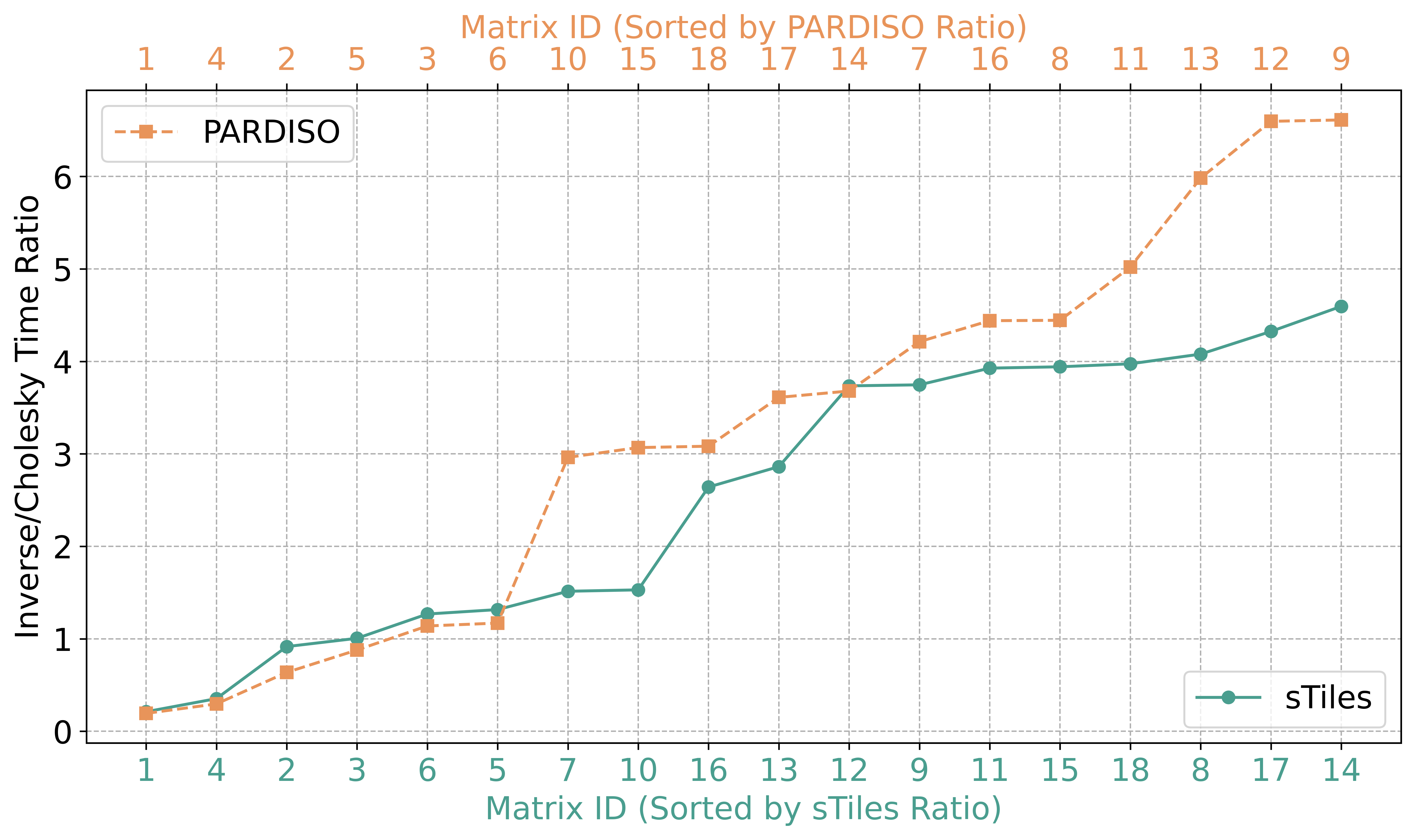
sTiles vs PARDISO for selected inversion on 500K matrices (computing (A⁻¹)ᵢⱼ on sparsity pattern)

sTiles vs PARDISO
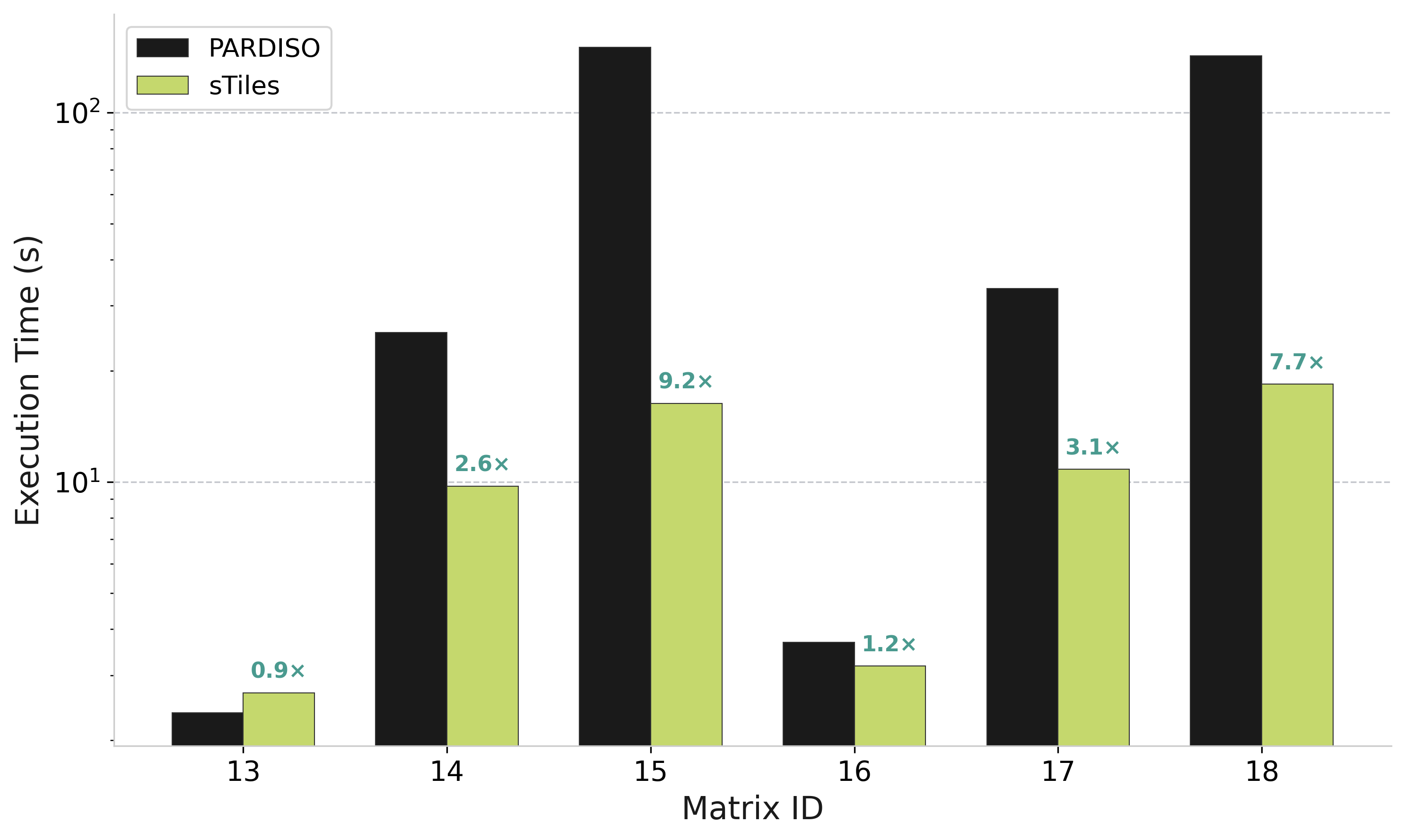
Selected Inversion Comparison

SelInv / Chol time ratio

SelInv over Chol ratio

Reference: PARDISO Selected Inversion [Schenk et al., SIAM SISC 2007]
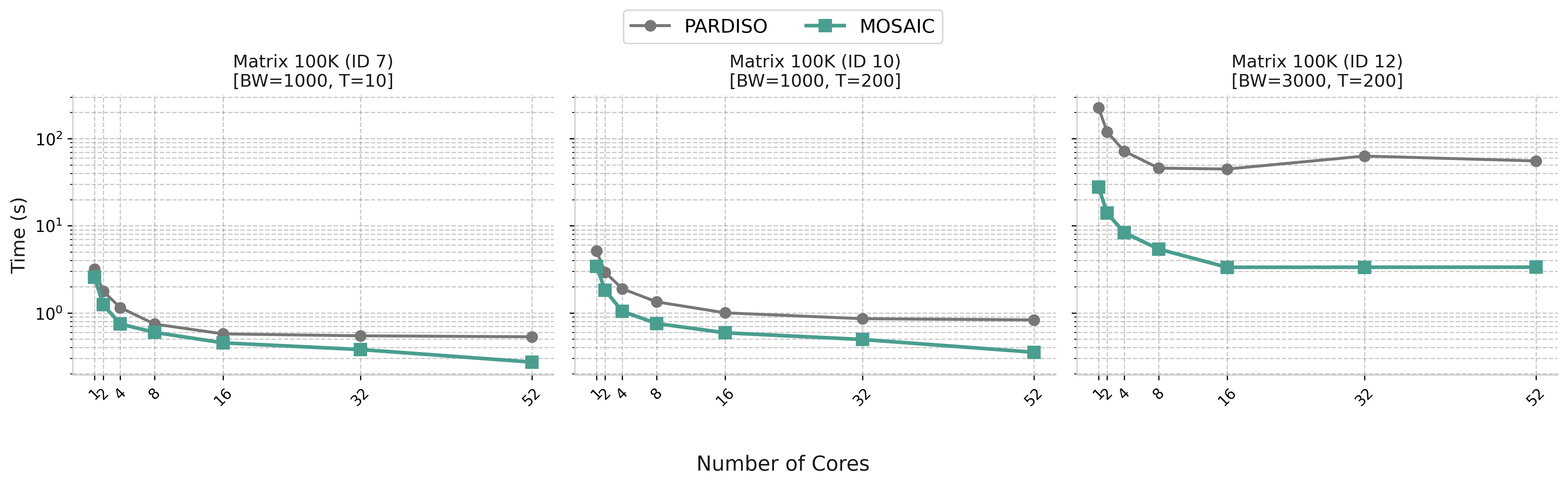
Scalability

Strong Scaling

AMD EPYC 7713 · 1-52 cores · 100K matrices

Key Observation

Matrix ID 12 (high bandwidth): 16× speedup at 52 cores. sTiles scales consistently while PARDISO saturates early.
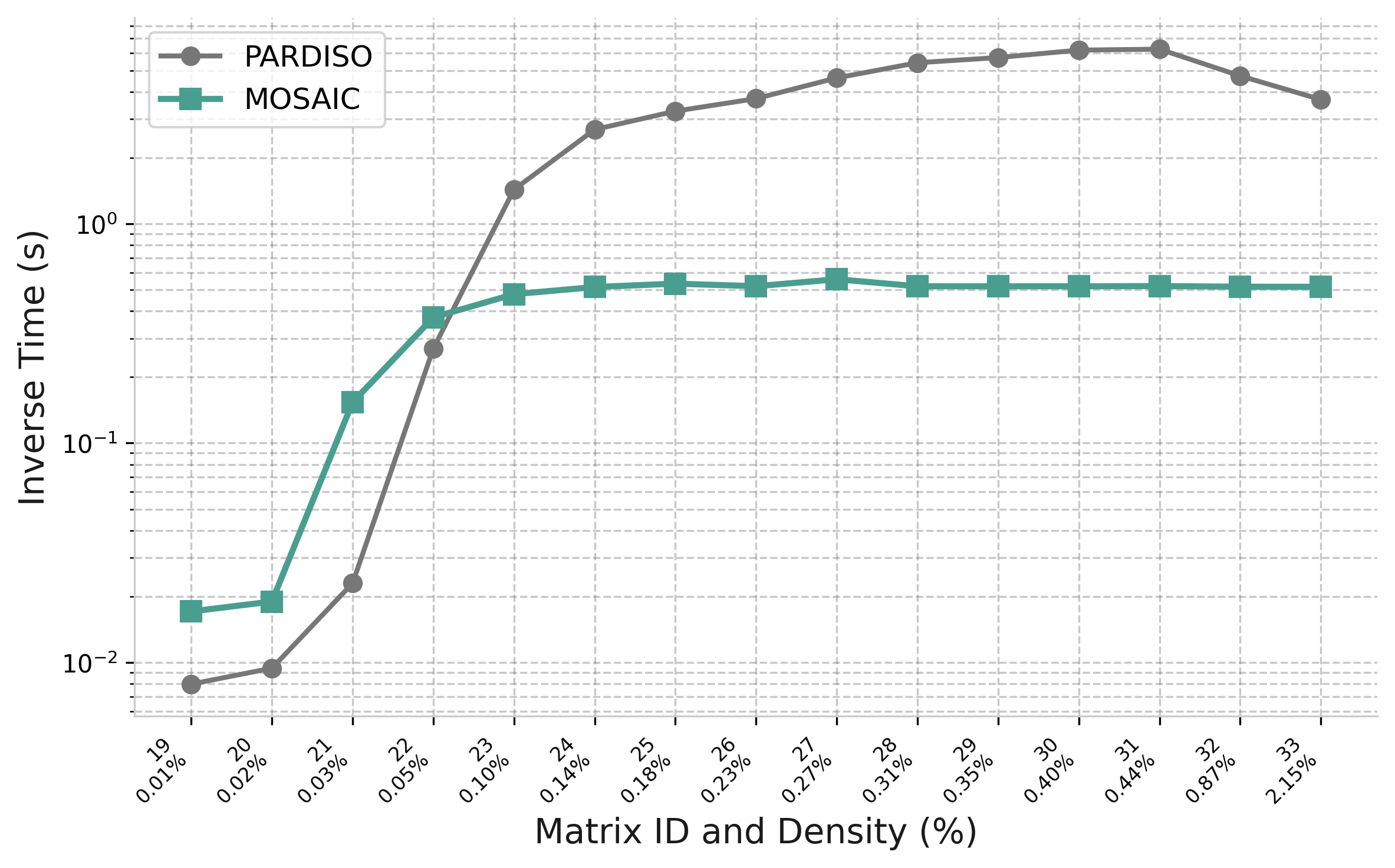
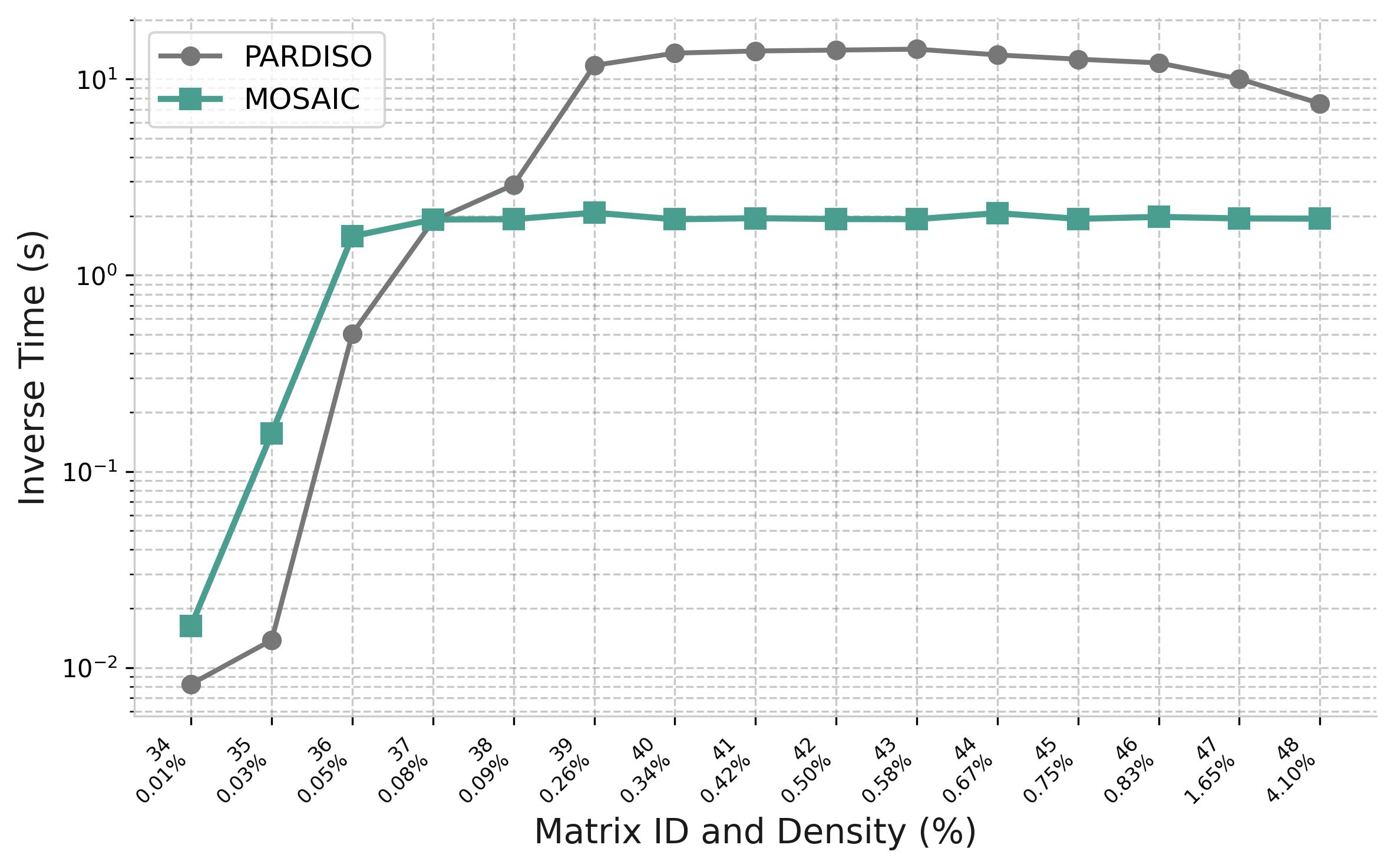
Impact of Sparsity

100K matrices · AMD EPYC 7713 · 52 cores

Bandwidth 1500

Bandwidth 3000

sTiles maintains stable performance across density levels · Up to 12× faster than PARDISO

Applicability

Non-Arrowhead Cases: General Sparse Matrices

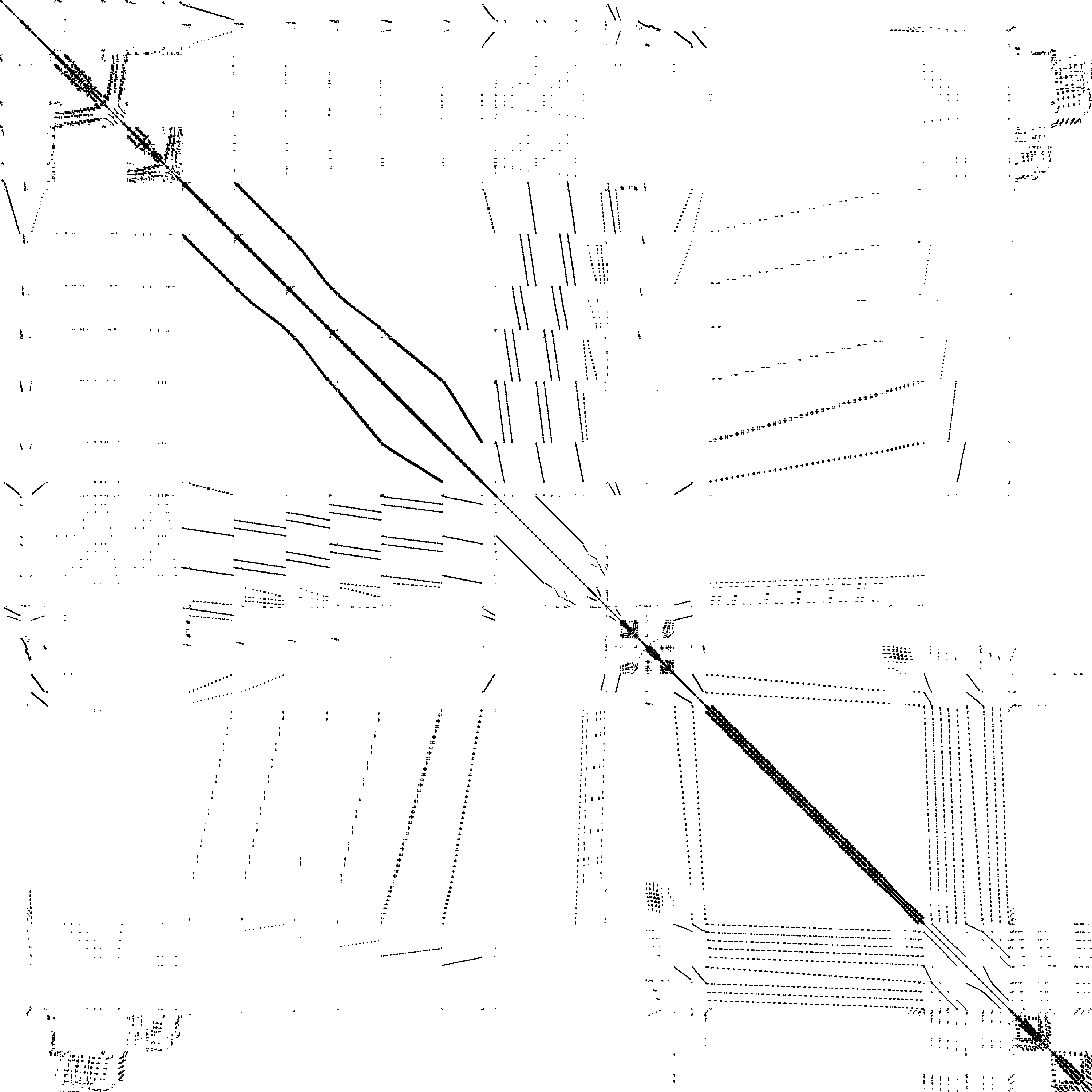
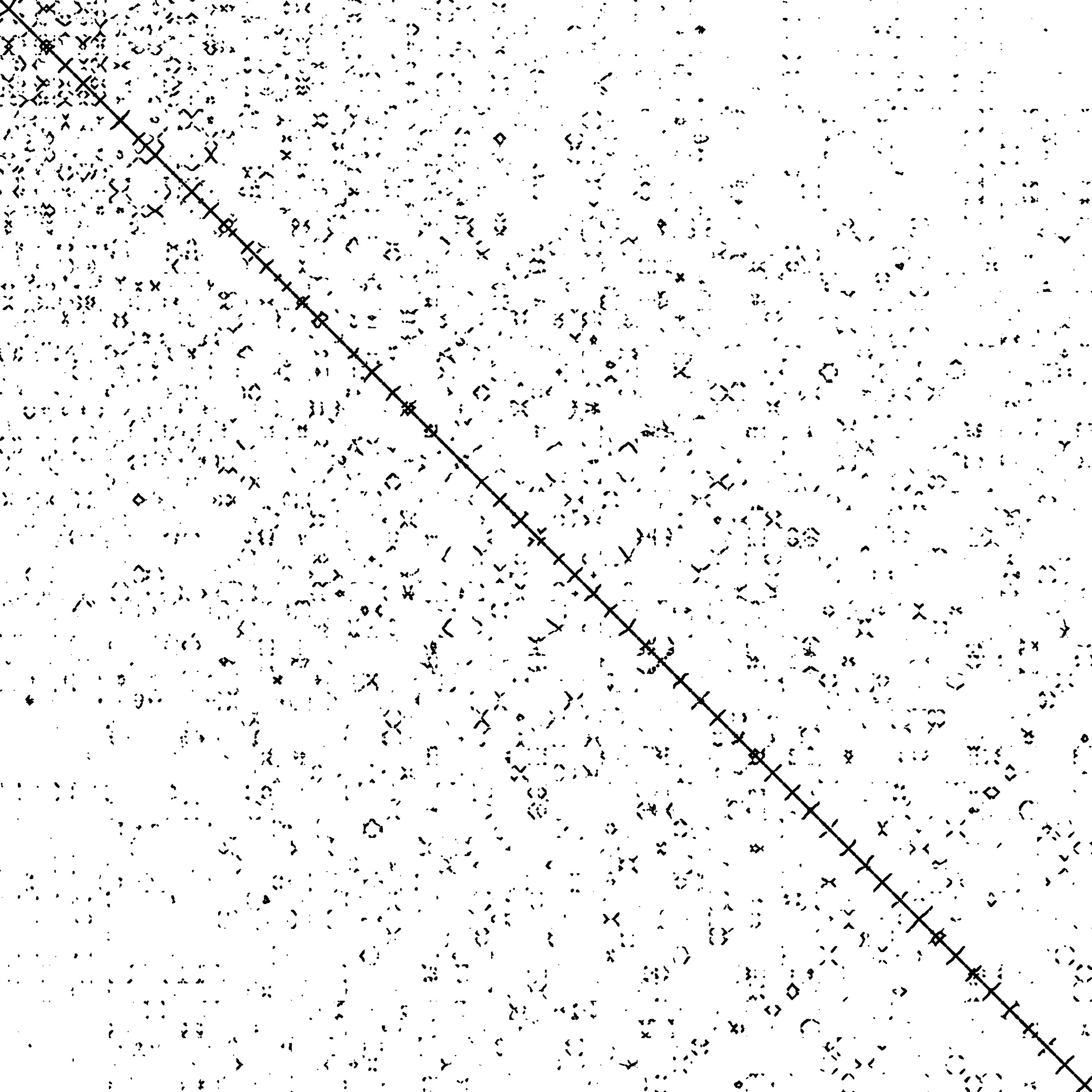
SuiteSparse matrices — sTiles tiling framework generalizes beyond arrowhead structure

ship_001

ship_001

n = 34,920  |  nnz = 3,896,496

# P-Chol P-SelInv S-Chol S-SelInv
10.3930.9060.5910.897
80.0800.2780.1040.270
160.0770.2890.0770.295
320.0640.3580.0890.326
500.0790.2840.0880.357
nd6k

nd6k

n = 18,000  |  nnz = 6,897,316

# P-Chol P-SelInv S-Chol S-SelInv
15.33510.5003.4796.360
80.8496.3540.5401.273
160.5505.6420.3510.934
320.4834.9720.4091.271
500.5524.1240.4561.320

GPU Acceleration

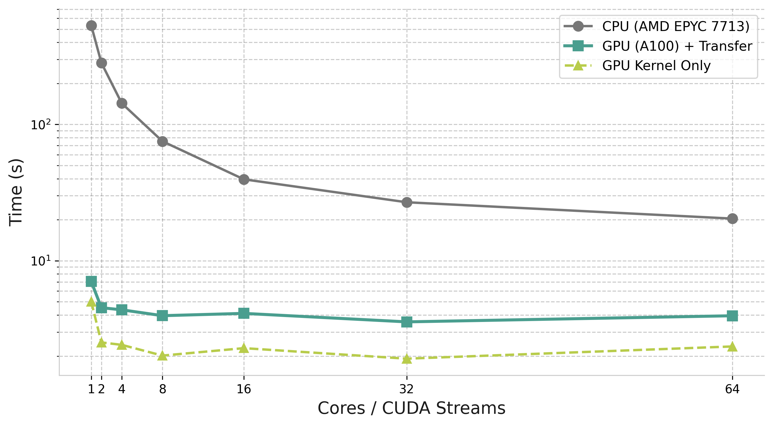
Matrix 50K · BW=15000 · NVIDIA A100 vs AMD EPYC 7713

5.7×
GPU vs 64-core CPU

GPU Implementation

  • Tile size 600 (vs 120 on CPU)
  • cuBLAS/cuSOLVER kernels
  • CUDA streams per host thread

Trade-off

Large tiles maximize kernel throughput but reduce task parallelism.

Conclusion

Summary

Contributions

  • Tile-based algorithm for selected inversion
  • Two-phase approach maximizing parallelism
  • GPU acceleration with cuBLAS/cuSOLVER

Key Results

  • Competitive with PARDISO; faster on high-bandwidth matrices
  • 5.7× faster on A100 vs 64-core EPYC
  • Stable across sparsity levels

Future Work

  • Multi-GPU support
  • Distributed memory systems

Impact

Enabling faster Bayesian inference for large-scale spatial statistics.

Thank You

Questions?

SIAM PP26 · March 2026
01 / 16